lesson 03
网格和运算符
网格是场景中的任何可见值 - 一个圆、一行文本、一个公式或其中任何一个的列表。大多数图表都是通过构造原始形状并应用运算符来设置它们的样式和位置来构建的。
>重要网格网格列表(或网格网格嵌套列表)称为网格树。大多数函数通过对每个组成网格进行操作来对网格树进行操作。
构造函数
构造函数在原点或原点附近创建几何体。操作员决定几何图形的走向和外观。这种分离使构造函数变得简单且可组合。
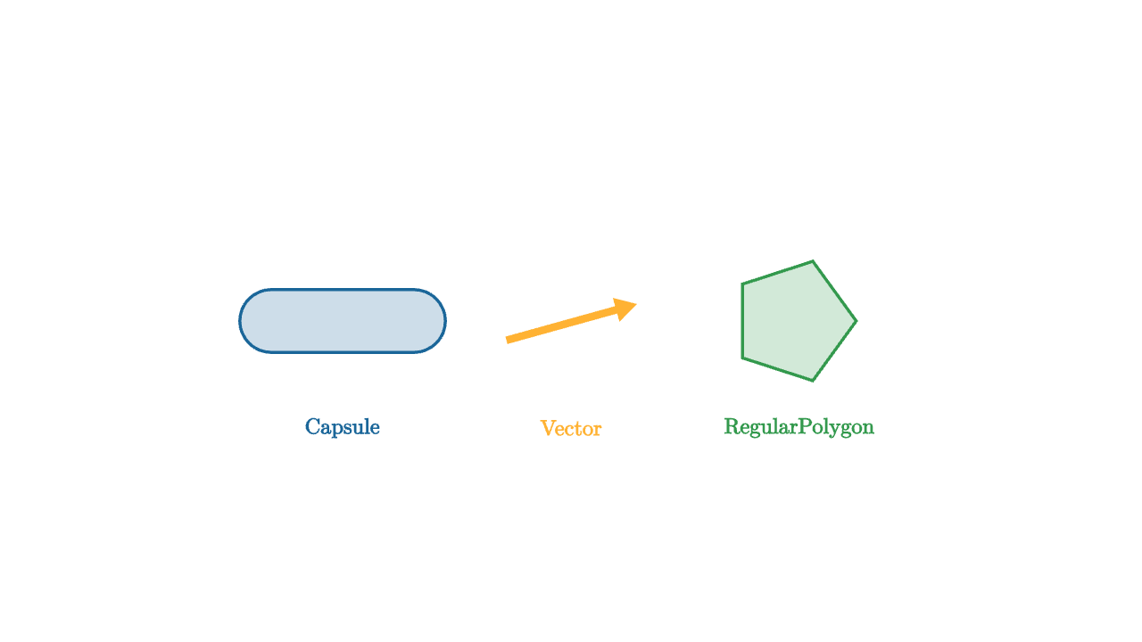
mesh demo = [
    center{1.6l} fill{soft{} BLUE} stroke{BLUE, 2} Capsule(0.5l, 0.5r, 0.22),
    center{ORIGIN} color{ORANGE} Vector(0.9r + 0.25u, 0.45l + 0.12d),
    center{1.6r} fill{soft{} GREEN} stroke{GREEN, 2} RegularPolygon(5, 0.44),
    center{1.6l + 0.75d} color{BLUE} Text("Capsule", 0.55),
    center{ORIGIN + 0.75d} color{ORANGE} Text("Vector", 0.55),
    center{1.6r + 0.75d} color{GREEN} Text("RegularPolygon", 0.55)
]
许多构造函数的列表供参考。请参阅文档以获取更多详细信息和选项。
Circle(radius)— XY 平面中的实心圆Annulus(inner, outer)— 带孔的填充环Square(width)— 中心正方形Rect([width, height])— 轴对齐矩形Arrow(start, end)— 带箭头的定向箭头Vector(delta, tail)— 从尾部到增量的箭头状向量Line(start, end)— 普通线段Polyline(vertices)— 通过点列表的开放路径Capsule(start, end, radius)— 圆形胶囊形状RegularPolygon(n, circumradius)— n 边多边形Arc(radius, [start_angle, end_angle])— 圆弧Triangle(p, q, r)— 三点三角形LineGrid(x_bounds, y_bounds)— 矩形线网格ColorGrid(color_at, x_bounds, y_bounds)— 采样的彩色网格Axis1d(...),Axis2d(...),Axis3d(...)— 坐标轴ExplicitFunc(func, [x_min, x_max, samples])— 函数曲线Field(glyph_func, x_bounds, y_bounds)— 在每个网格点重复字形Label(target, string, direction)— TeX 标签放置在网格旁边Text(string, size)— 渲染文本Tex(string_or_list, size)— 渲染的 LaTeX 公式Dot(point)— 单个面向屏幕的点
样式操作符
操作员将网格变换到右侧。样式操作符设置视觉属性。
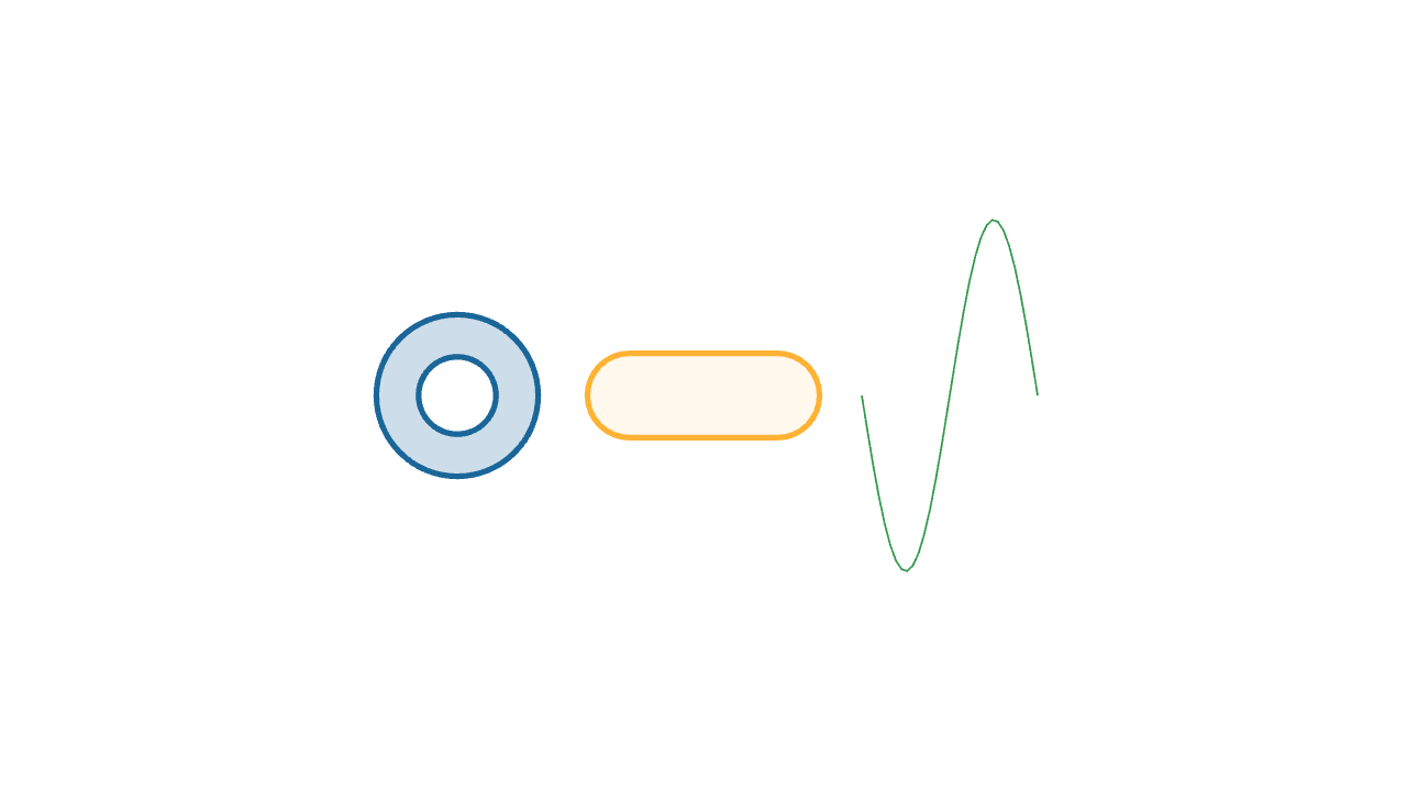
mesh demo = [
    center{1.4l} fill{soft{} BLUE} stroke{BLUE, 3} Annulus(0.22, 0.46),
    center{0r} fill{alpha{0.4} soft{} ORANGE} stroke{ORANGE, 3} Capsule(0.42l, 0.42r, 0.24),
    center{1.4r} color{GREEN} ExplicitFunc(|x| sin(x * TAU), [-0.5, 0.5, 32])
]fill{color}— 填充闭合网格的内部stroke{color, width}— 用彩色描边勾勒出网格的轮廓color{color}— 设置描边和填充alpha{opacity}— 缩放网格的透明度;适用于其右侧的任何内容scale{factor}— 统一比例尺;或每轴scale{[sx, sy, sz]}
定位算子
定位算子将网格放置在空间中。
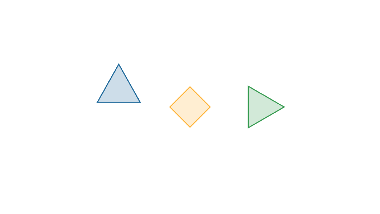
mesh demo = [
    center{1.5l + 0.5u} fill{soft{} BLUE} stroke{BLUE, 2} Triangle(0.45l + 0.35d, 0.45r + 0.35d, 0.45u),
    center{0r} rotate{PI / 4} fill{soft{} ORANGE} stroke{ORANGE, 2} Square(0.6),
    shift{1.5r} scale{1.2} fill{soft{} GREEN} stroke{GREEN, 2} RegularPolygon(3, 0.42)
]center{position}— 移动网格,使其边界框中心位于positionshift{delta}— 将网格平移矢量偏移量rotate{angle}— 绕 Z 轴旋转(或传递全轴矢量)in_space{origin, x_basis, y_basis}— 将网格放置在局部坐标系中
布局运算符
布局运算符将一个网格相对于另一个网格定位,因此不需要对坐标进行硬编码。
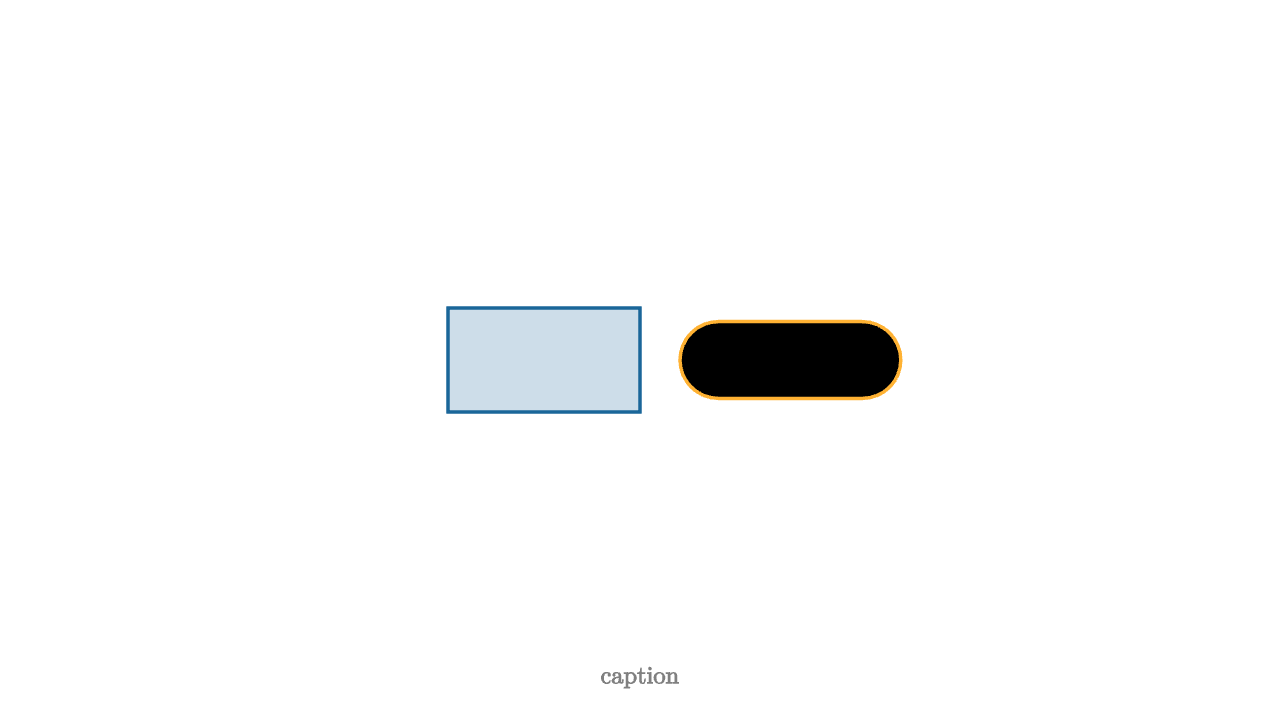
let box = center{0.6l} fill{soft{} BLUE} stroke{BLUE, 2} Rect([1.2, 0.65])

mesh demo = [
    box,
    next_to{box, 1r, 0.25} stroke{ORANGE, 2} Capsule(0.45l, 0.45r, 0.24),
    to_side{1d, 0.2} color{GRAY} Text("caption", 0.55)
]
next_to{base, direction, spacing}— 沿着direction将网格放置在base旁边to_side{direction, spacing}— 将网格放置在可见帧的边缘附近
自定义运算符
当多个网格共享一个视觉配方时,将其提取到一个运算符中。
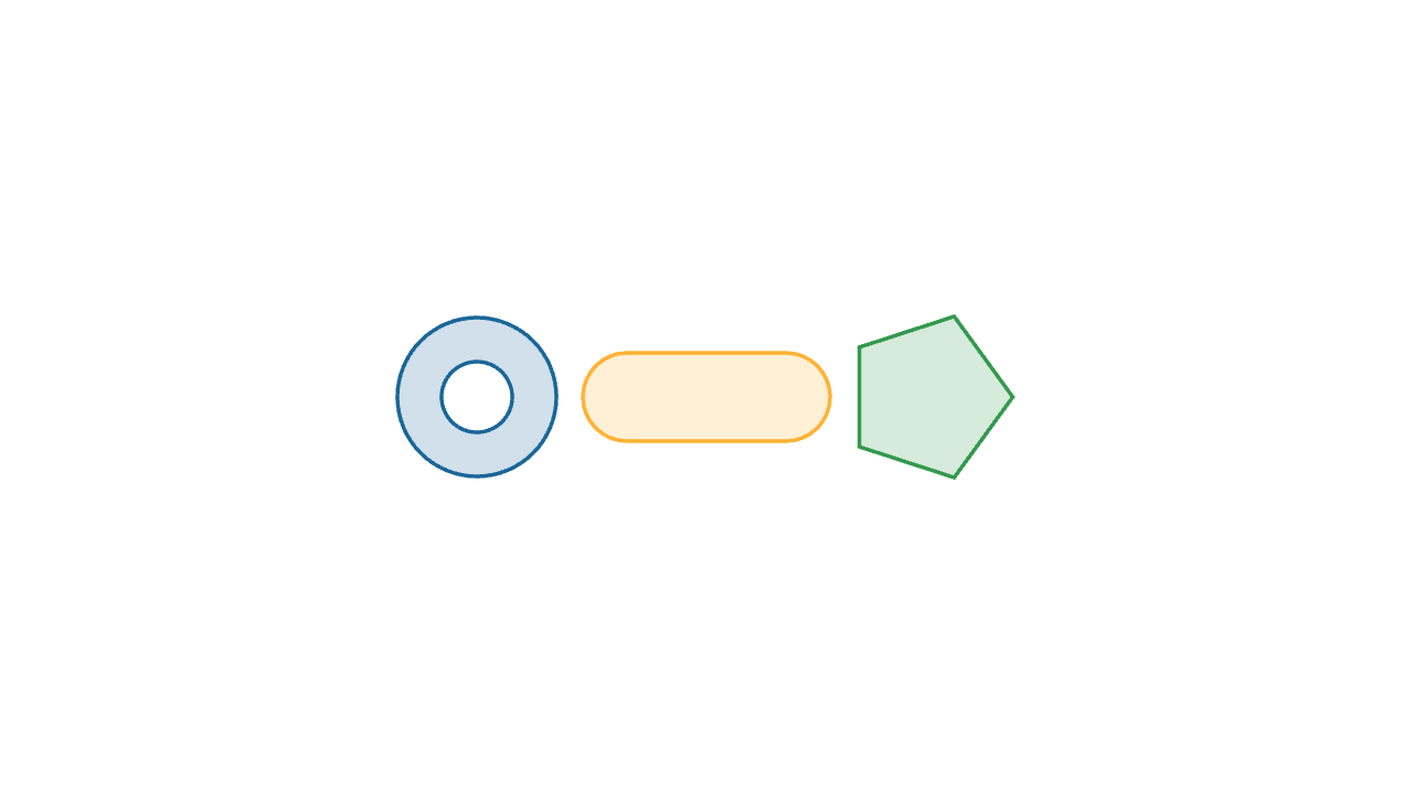
let soft_style = operator |target, col|
fill{alpha{0.2} col}
stroke{col, 2}
target
mesh demo = [
center{1.3l} soft_style{BLUE} Annulus(0.2, 0.45),
center{0r} soft_style{ORANGE} Capsule(0.45l, 0.45r, 0.25),
center{1.3r} soft_style{GREEN} RegularPolygon(5, 0.48)
]
"custom"
play Grow(1)网状树
回想一下,网格树列表本身就是一棵网格树。这就是大多数图表的组装方式。
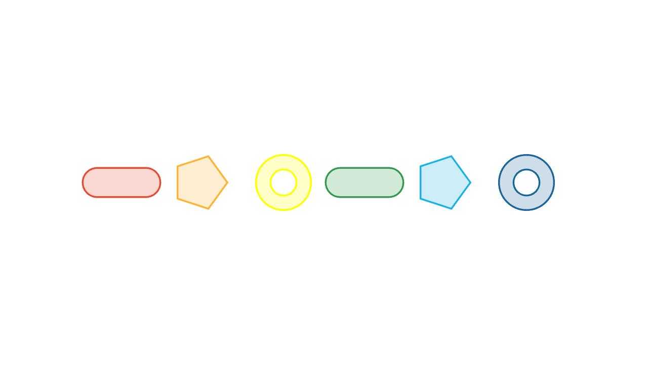
let Row = |items| block {
    for (i in range(0, len(items))) {
        let x = (i - (len(items) - 1) / 2) * 1.0
        let kind = mod(i, 3)
        var shape = []
        if (kind == 0) {
            shape = Capsule(0.3l, 0.3r, 0.18)
        } else if (kind == 1) {
            shape = RegularPolygon(5, 0.34)
        } else {
            shape = Annulus(0.16, 0.34)
        }
        . center{[x, 0, 0]} fill{soft{} items[i]} stroke{items[i], 2} shape
    }
}

mesh demo = Row([RED, ORANGE, YELLOW, GREEN, CYAN, BLUE])
使用 block {} 和 .= 循环构建网格是数据驱动图的标准模式。
标签和过滤器
>重要标签通过为网格体分配一个数字列表(默认情况下为 []),将身份附加到网格体上。然后,过滤器和运算符可以设计或隔离标记的子集。
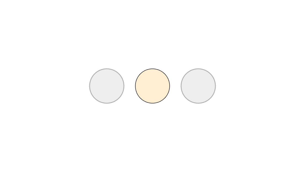
let muted = |tags| not (2 in tags)

mesh demo =
    fill{soft{} LIGHT_GRAY, muted} # only applies to edge meshes!
    stroke{LIGHT_GRAY, 2, muted}
    [
        tag{1} center{1.2l} fill{soft{} BLUE} Circle(0.45),
        tag{2} center{0r} fill{soft{} ORANGE} Circle(0.45),
        tag{3} center{1.2r} fill{soft{} GREEN} Circle(0.45)
    ]

# selects a subset of the input
let edges = tag_filter{muted} demo
过滤器 |tags| not (2 in tags) 匹配标签集不包含 2 的任何片段。 fill 和 stroke 运算符使用此过滤器仅设置静音片段的样式,使橙色圆圈保持全彩。
当片段需要在转换过程中保持其身份时,标签在动画中变得很重要。
文本和 TeX
Text 和 Tex 生成网格就像任何几何构造函数一样。可以使用相同的操作符和动画对它们进行样式设置、定位、标记和动画处理。
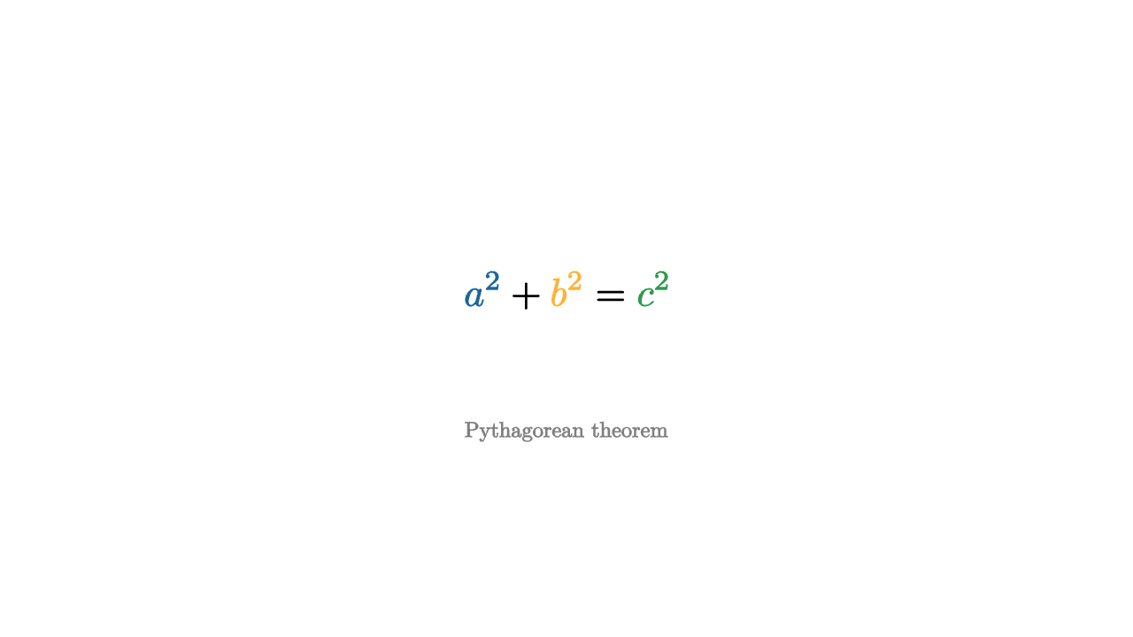
let palette = operator |target|
color{BLUE, |tag| 1 in tag}
color{ORANGE, |tag| 2 in tag}
color{GREEN, |tag| 3 in tag}
target
mesh formula = center{0.2u} palette{} Tex([
text_tag{1} "a^2",
" + ",
"\text_tag{2}{b^2}",
" = ",
"\tag3{c^2}" # all three are valid ways to tagging tect
], 1.0)
mesh caption = center{0.8d} color{GRAY} Text("Pythagorean theorem", 0.55)
"formula"
play [Write(1, [&formula]), Fade(0.8, [&caption])]text_tag{} 是 tag{} 的文本对应项。它赋予公式的各个部分稳定的身份。它在内部扩展为字符串 \text_tag{tags}{text},并由 \tag1{}、\tag2{} 等别名。
工作示例
函数图
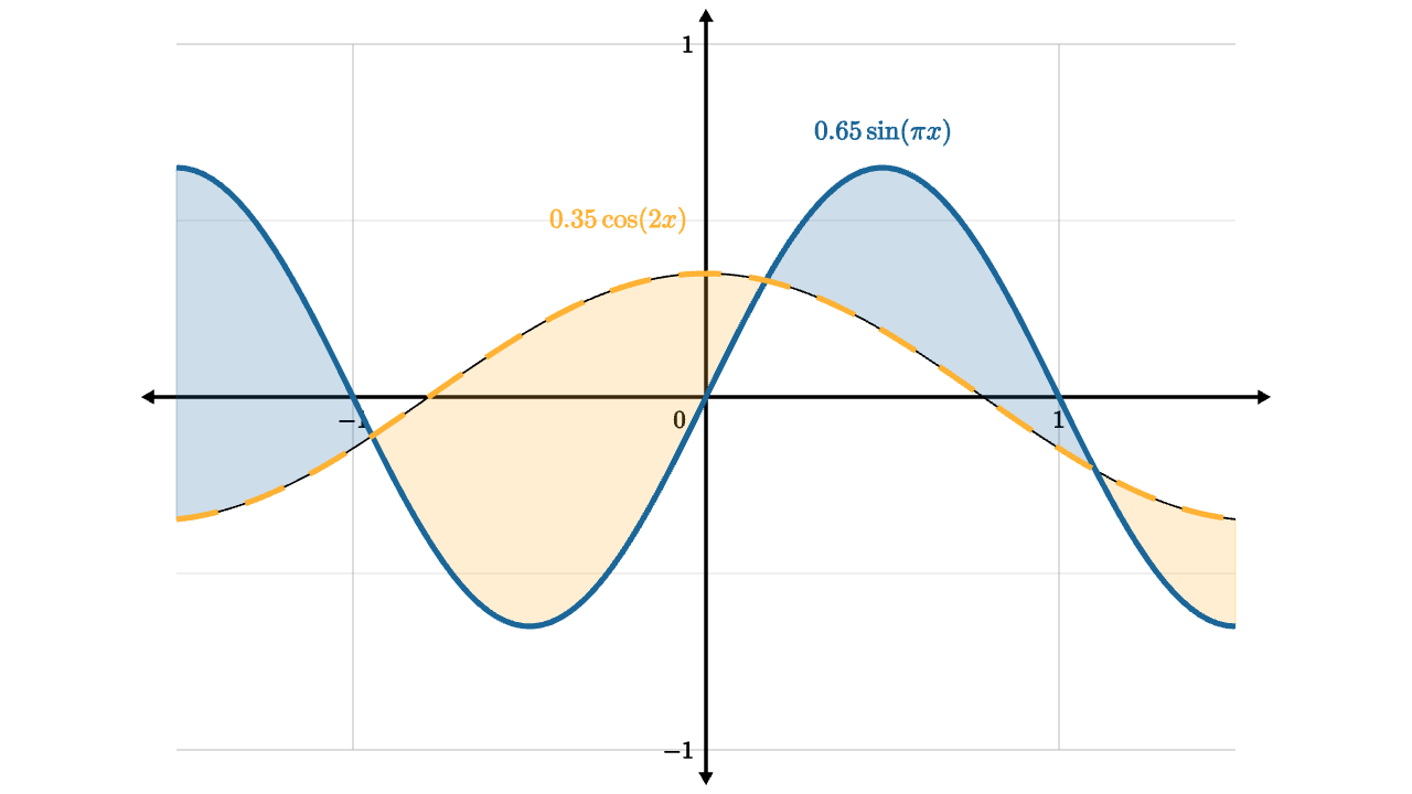
let unit = 2
let f = |x| 0.65 * sin(x * PI)
let g = |x| 0.35 * cos(2 * x)
let graph_space = operator |target|
    in_space{0l, unit * 1r, unit * 1u}
    target

let sine = z_index{2} graph_space{} stroke{BLUE, 3} ExplicitFunc(f, [-1.5, 1.5, 120])
let cosine = z_index{2} graph_space{} stroke{ORANGE, 3} dashed{[0.12, 0.08]} ExplicitFunc(g, [-1.5, 1.5, 120])
let area =
    z_index{1}
    graph_space{}
    ExplicitFuncDiff(
        f,
        g,
        [-1.5, 1.5, 120],
        [alpha{0.22} BLUE, alpha{0.22} ORANGE],
        [[1], [2]]
    )

mesh plot = [
    axis_style{"x", -1.5, 1.5, nil, 1, 1}
    axis_style{"y", -1, 1, nil, 0.5, 2}
    Axis2d([unit * 1r, unit * 1u], BLACK, LIGHT_GRAY),
    area,
    sine,
    cosine,
    color{BLUE} center{1.5u + 1r} Tex("0.65 \sin(\pi x)", 0.55),
    color{ORANGE} center{1u + 0.5l} Tex("0.35 \cos(2x)", 0.55)
]
矢量场
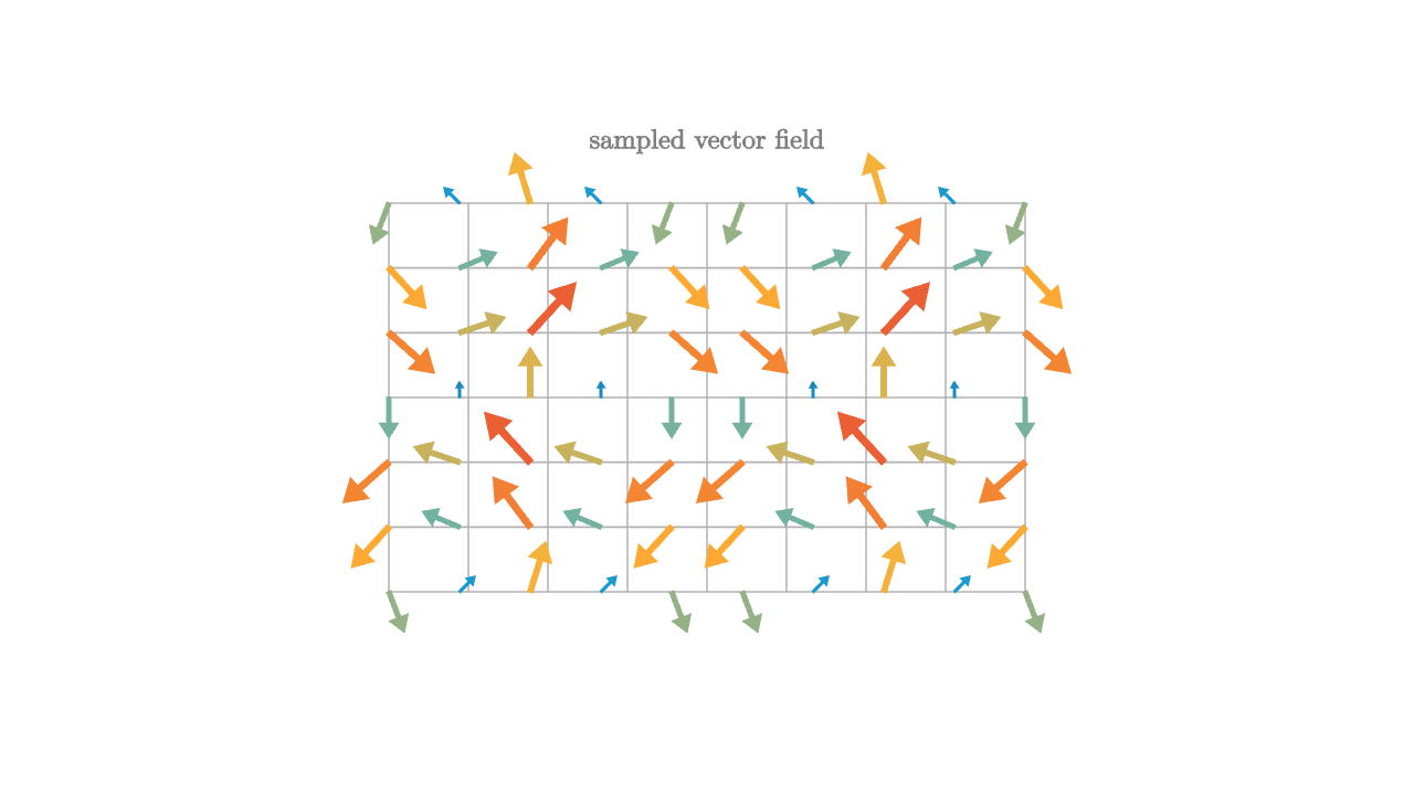
let palette = [0 -> BLUE, 0.45 -> CYAN, 0.75 -> ORANGE, 1 -> RED]

let Needle = |pos, idx| {
    let vx = sin(pos[1] * PI)
    let vy = -cos(pos[0] * PI)
    let strength = norm([vx, vy, 0])
    let col = keyframe_lerp(palette, strength / 1.42)
    return color{col} Vector(0.28 * [vx, vy, 0], pos)
}

mesh grid = stroke{LIGHT_GRAY, 1} LineGrid([-1.8, 1.8, 9], [-1.1, 1.1, 7])
mesh field = Field(Needle, [-1.8, 1.8, 10], [-1.1, 1.1, 7])
mesh center_dot = fill{BLACK} Dot(ORIGIN)
mesh title = center{1.45u} color{GRAY} Text("sampled vector field", 0.55)
3D表面
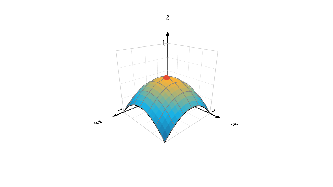
let h = |x, y| 1.2 * (0.5 - (x - 0.5)^2 - (y - 0.5)^2)
let keys = [0 -> BLUE, 0.3 -> CYAN, 0.6 -> ORANGE, 1 -> RED]
let col_at = |pos, idx| keyframe_lerp(keys, h(pos[0], -pos[1]))

# here in space would just be a negation, so we do it manually
mesh surface =
    stroke{BLACK, 1}
    point_map{|p| [p[0], p[1], h(p[0], -p[1])]}
    ColorGrid(col_at, [0, 1, 18], [-1, 0, 18])

mesh wire =
    stroke{GRAY, 1}
    point_map{|p| [p[0], p[1], h(p[0], -p[1]) + 0.01]}
    LineGrid([0, 1, 7], [-1, 0, 7])

mesh axis =
    axis_style{"x", 0, 1, "x"}
    axis_style{"y", 0, 1, "y"}
    axis_style{"z", 0, 1, "z"}
    Axis3d(basis: [1r, 1d, 1b], color: BLACK, grid_color: LIGHT_GRAY, [1u, 1u, 1b])

mesh peak = color{RED} shift{pos:[0.5, -0.5, h(0.5, 0.5)]} Sphere(0.05)

camera = Camera([2.2, -2.1, 1.45], [0.5, -0.5, 0.35], [0, 0, 1])