lesson 03
Meshes And Operators
A mesh is any visible value in a scene — a circle, a line of text, a formula, or a list of any of those. Most diagrams are built by constructing primitive shapes and applying operators to style and position them.
Constructors
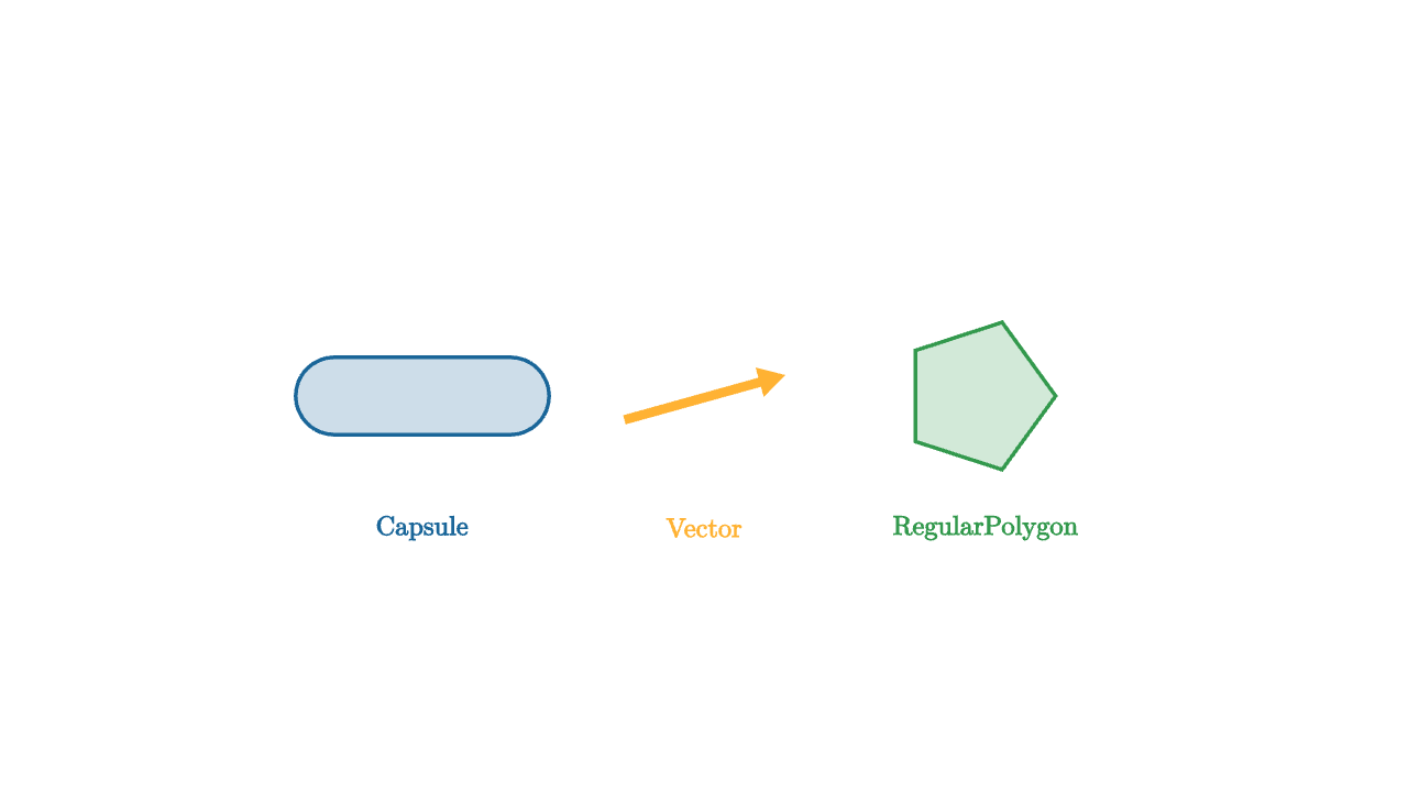
Constructors create geometry at or near the origin. Operators decide where geometry goes and how it looks. The separation keeps constructors simple and composable.
let soft = |col| lerp(WHITE, col, 0.22)

mesh demo = [
    center{1.6l} fill{soft(BLUE)} stroke{BLUE, 2} Capsule(0.5l, 0.5r, 0.22),
    center{ORIGIN} color{ORANGE} Vector(0.9r + 0.25u, 0.45l + 0.12d),
    center{1.6r} fill{soft(GREEN)} stroke{GREEN, 2} RegularPolygon(5, 0.44),
    center{1.6l + 0.75d} color{BLUE} Text("Capsule", 0.55),
    center{ORIGIN + 0.75d} color{ORANGE} Text("Vector", 0.55),
    center{1.6r + 0.75d} color{GREEN} Text("RegularPolygon", 0.55)
]
A list of many constructors for reference. Look at documentation for more details and options.
Circle(radius)— filled circle in the XY planeAnnulus(inner, outer)— filled ring with a holeSquare(width)— centered squareRect([width, height])— axis-aligned rectangleArrow(start, end)— directed arrow with arrowheadVector(delta, tail)— arrow-like vector from a tail by a deltaLine(start, end)— plain line segmentPolyline(vertices)— open path through a list of pointsCapsule(start, end, radius)— rounded capsule shapeRegularPolygon(n, circumradius)— n-sided polygonArc(radius, [start_angle, end_angle])— circular arcTriangle(p, q, r)— three-point triangleLineGrid(x_bounds, y_bounds)— rectangular line gridColorGrid(color_at, x_bounds, y_bounds)— sampled colored gridAxis1d(...),Axis2d(...),Axis3d(...)— coordinate axesExplicitFunc(func, [x_min, x_max, samples])— curve from a functionField(glyph_func, x_bounds, y_bounds)— repeating glyph at each grid pointLabel(target, string, direction)— TeX label placed beside a meshText(string, size)— rendered textTex(string_or_list, size)— rendered LaTeX formulaDot(point)— single screen-facing point
Styling Operators
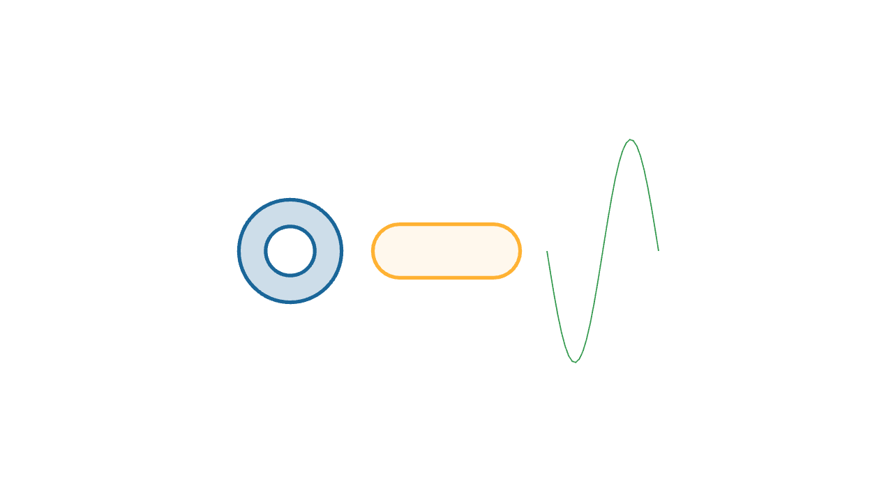
Operators transform the mesh to their right. Styling operators set visual properties.
let soft = |col| lerp(WHITE, col, 0.22)

mesh demo = [
    center{1.4l} fill{soft(BLUE)} stroke{BLUE, 3} Annulus(0.22, 0.46),
    center{0r} fill{alpha{0.4} soft(ORANGE)} stroke{ORANGE, 3} Capsule(0.42l, 0.42r, 0.24),
    center{1.4r} color{GREEN} ExplicitFunc(|x| sin(x * TAU), [-0.5, 0.5, 32])
]fill{color}— fills the interior of a closed meshstroke{color, width}— outlines the mesh with a colored strokecolor{color}— sets stroke and fillalpha{opacity}— scales the transparency of the mesh; applies to whatever is to its rightscale{factor}— uniform scale; orscale{[sx, sy, sz]}per-axis
Positioning Operators
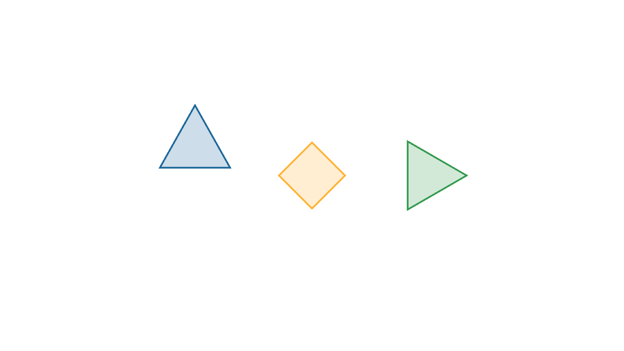
Positioning operators place meshes in space.
let soft = |col| lerp(WHITE, col, 0.22)

mesh demo = [
    center{1.5l + 0.5u} fill{soft(BLUE)} stroke{BLUE, 2} Triangle(0.45l + 0.35d, 0.45r + 0.35d, 0.45u),
    center{0r} rotate{PI / 4} fill{soft(ORANGE)} stroke{ORANGE, 2} Square(0.6),
    shift{1.5r} scale{1.2} fill{soft(GREEN)} stroke{GREEN, 2} RegularPolygon(3, 0.42)
]center{position}— moves the mesh so its bounding-box center is atpositionshift{delta}— translates the mesh by a vector offsetrotate{angle}— rotates around the Z axis (or pass a full axis vector)in_space{origin, x_basis, y_basis}— places the mesh in a local coordinate frame
Layout Operators
Layout operators position one mesh relative to another, so coordinates do not need to be hardcoded.
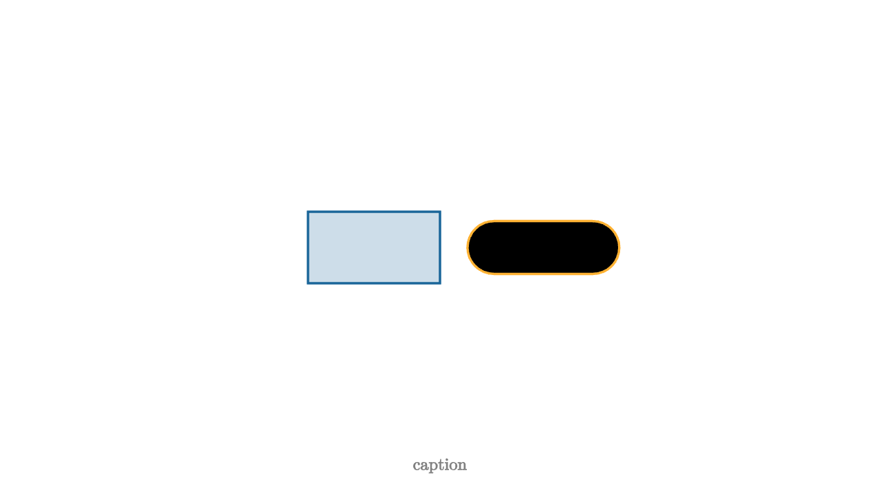
let soft = |col| lerp(WHITE, col, 0.22)

let box = center{0.6l} fill{soft(BLUE)} stroke{BLUE, 2} Rect([1.2, 0.65])

mesh demo = [
    box,
    next_to{box, 1r, 0.25} stroke{ORANGE, 2} Capsule(0.45l, 0.45r, 0.24),
    to_side{1d, 0.2} color{GRAY} Text("caption", 0.55)
]
next_to{base, direction, spacing}— positions a mesh next tobasealongdirectionto_side{direction, spacing}— positions a mesh near the edge of the visible frame
Custom Operators
When multiple meshes share a visual recipe, extract it into an operator.
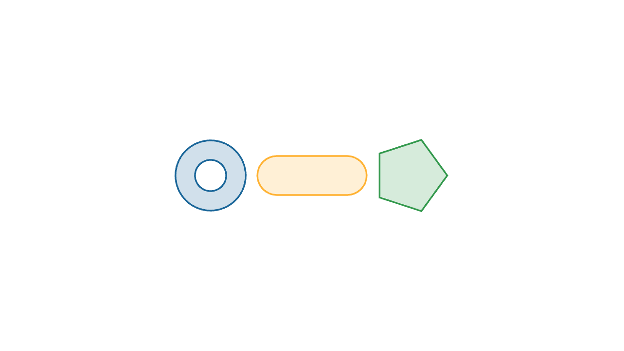
let soft_style = operator |target, col|
fill{alpha{0.2} col}
stroke{col, 2}
target
mesh demo = [
center{1.3l} soft_style{BLUE} Annulus(0.2, 0.45),
center{0r} soft_style{ORANGE} Capsule(0.45l, 0.45r, 0.25),
center{1.3r} soft_style{GREEN} RegularPolygon(5, 0.48)
]
"custom"
play Grow(1)Mesh Trees
Recall that a list of mesh trees is itself a mesh tree. This is how most diagrams are assembled.
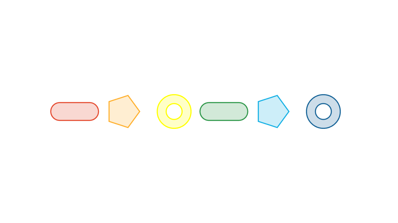
let soft = |col| lerp(WHITE, col, 0.22)

let Row = |items| block {
    for (i in range(0, len(items))) {
        let x = (i - (len(items) - 1) / 2) * 1.0
        let kind = mod(i, 3)
        var shape = []
        if (kind == 0) {
            shape = Capsule(0.3l, 0.3r, 0.18)
        } else if (kind == 1) {
            shape = RegularPolygon(5, 0.34)
        } else {
            shape = Annulus(0.16, 0.34)
        }
        . center{[x, 0, 0]} fill{soft(items[i])} stroke{items[i], 2} shape
    }
}

mesh demo = Row([RED, ORANGE, YELLOW, GREEN, CYAN, BLUE])
Building meshes in loops with block {} and .= is the standard pattern for data-driven diagrams.
Tags And Filters
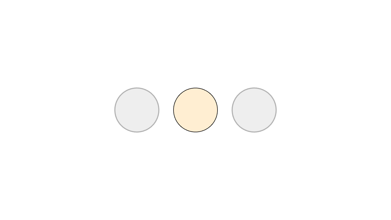
let soft = |col| lerp(WHITE, col, 0.22)

let muted = |tags| not (2 in tags)

mesh demo =
    fill{soft(LIGHT_GRAY), muted} # only applies to edge meshes!
    stroke{LIGHT_GRAY, 2, muted}
    [
        tag{1} center{1.2l} fill{soft(BLUE)} Circle(0.45),
        tag{2} center{0r} fill{soft(ORANGE)} Circle(0.45),
        tag{3} center{1.2r} fill{soft(GREEN)} Circle(0.45)
    ]

# selects a subset of the input
let edges = tag_filter{muted} demo
The filter |tags| not (2 in tags) matches any fragment whose tag set does not include 2. The fill and stroke operators use this filter to style only the muted fragments, leaving the orange circle at full color.
Tags become important in animation when pieces need to keep their identity across a transformation.
Text And TeX
Text and Tex produce meshes just like any geometric constructor. They can be styled, positioned, tagged, and animated with the same operators and animations.
let palette = operator |target|
color{BLUE, |tag| 1 in tag}
color{ORANGE, |tag| 2 in tag}
color{GREEN, |tag| 3 in tag}
target
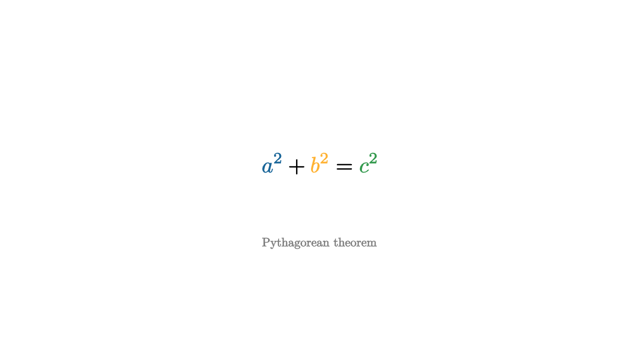
mesh formula = center{0.2u} palette{} Tex([
text_tag{1} "a^2",
" + ",
"\text_tag{2}{b^2}",
" = ",
"\tag3{c^2}" # all three are valid ways to tagging tect
], 1.0)
mesh caption = center{0.8d} color{GRAY} Text("Pythagorean theorem", 0.55)
"formula"
play [Write(1, [&formula]), Fade(0.8, [&caption])]text_tag{} is the text counterpart to tag{}. It gives individual pieces of a formula stable identity. It internally expands to the string \text_tag{tags}{text}, and is aliased by \tag1{}, \tag2{}, etc.
Worked Examples
Function Plot
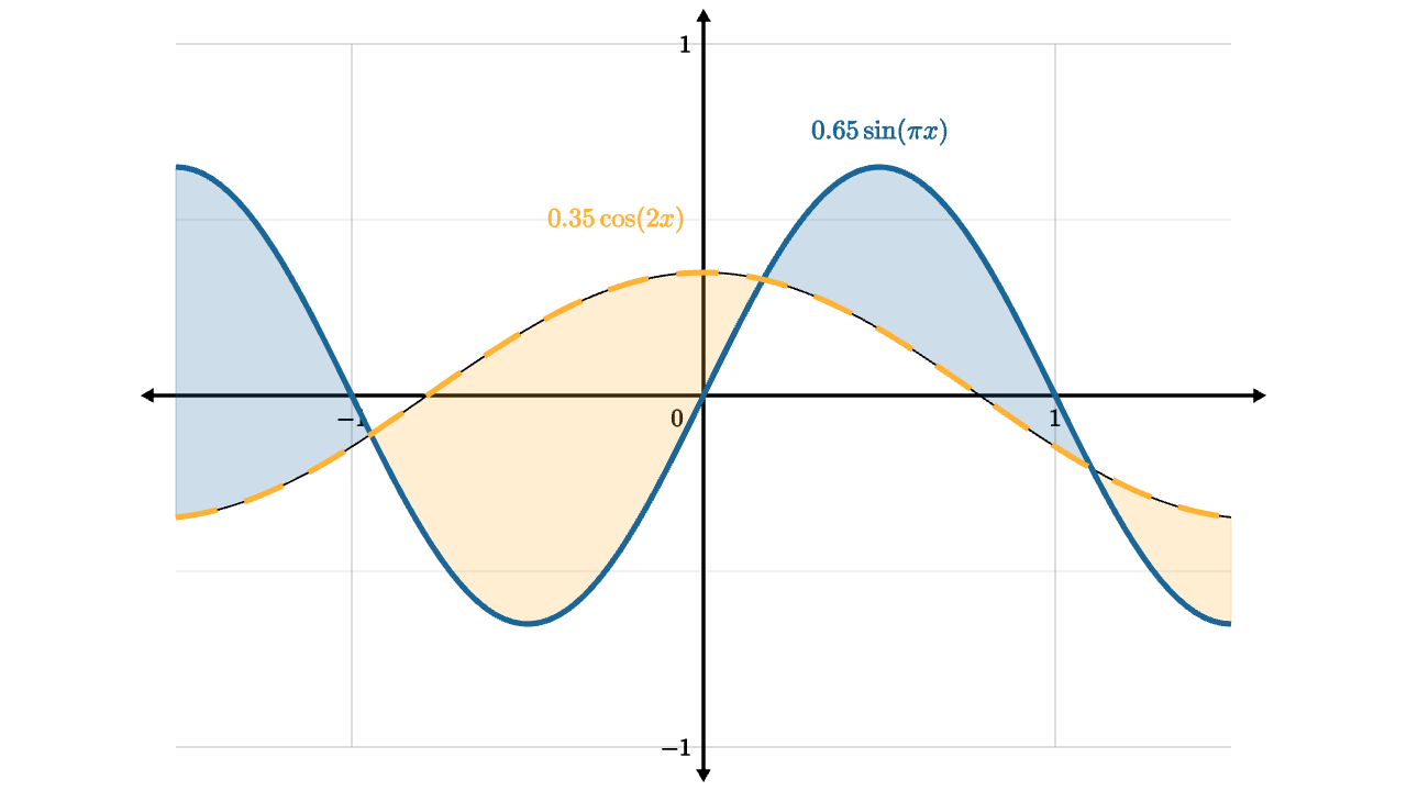
let unit = 2
let f = |x| 0.65 * sin(x * PI)
let g = |x| 0.35 * cos(2 * x)
let graph_space = operator |target|
    in_space{0l, unit * 1r, unit * 1u}
    target

let sine = z_index{2} graph_space{} stroke{BLUE, 3} ExplicitFunc(f, [-1.5, 1.5, 120])
let cosine = z_index{2} graph_space{} stroke{ORANGE, 3} dashed{[0.12, 0.08]} ExplicitFunc(g, [-1.5, 1.5, 120])
let area =
    z_index{1}
    graph_space{}
    ExplicitFuncDiff(
        f,
        g,
        [-1.5, 1.5, 120],
        [alpha{0.22} BLUE, alpha{0.22} ORANGE],
        [[1], [2]]
    )

mesh plot = [
    axis_style{"x", -1.5, 1.5, nil, 1, 1}
    axis_style{"y", -1, 1, nil, 0.5, 2}
    Axis2d([unit * 1r, unit * 1u], BLACK, LIGHT_GRAY),
    area,
    sine,
    cosine,
    color{BLUE} center{1.5u + 1r} Tex("0.65 \sin(\pi x)", 0.55),
    color{ORANGE} center{1u + 0.5l} Tex("0.35 \cos(2x)", 0.55)
]
Vector Field
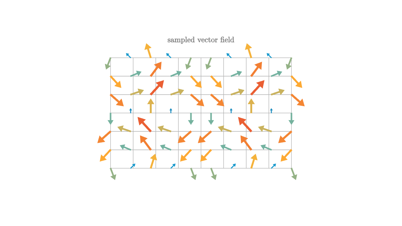
let palette = [0 -> BLUE, 0.45 -> CYAN, 0.75 -> ORANGE, 1 -> RED]

let Needle = |pos, idx| {
    let vx = sin(pos[1] * PI)
    let vy = -cos(pos[0] * PI)
    let strength = norm([vx, vy, 0])
    let col = keyframe_lerp(palette, strength / 1.42)
    return color{col} Vector(0.28 * [vx, vy, 0], pos)
}

mesh grid = stroke{LIGHT_GRAY, 1} LineGrid([-1.8, 1.8, 9], [-1.1, 1.1, 7])
mesh field = Field(Needle, [-1.8, 1.8, 10], [-1.1, 1.1, 7])
mesh center_dot = fill{BLACK} Dot(ORIGIN)
mesh title = center{1.45u} color{GRAY} Text("sampled vector field", 0.55)
3D Surface
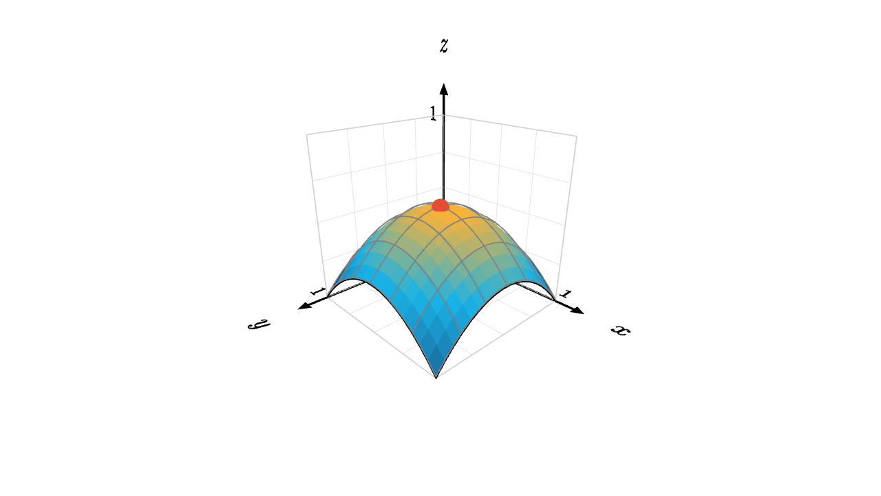
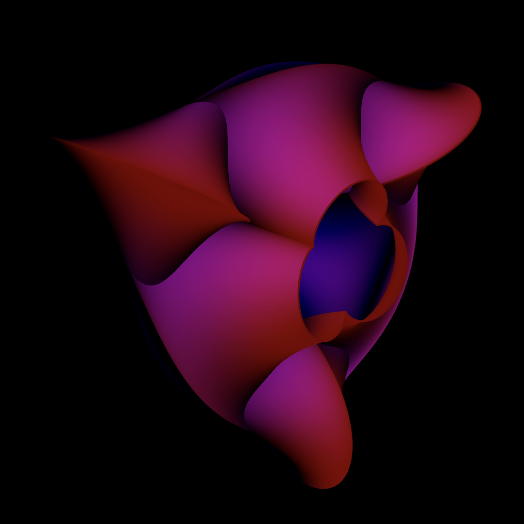
let h = |x, y| 1.2 * (0.5 - (x - 0.5)^2 - (y - 0.5)^2)
let keys = [0 -> BLUE, 0.3 -> CYAN, 0.6 -> ORANGE, 1 -> RED]
let col_at = |pos, idx| keyframe_lerp(keys, h(pos[0], -pos[1]))

# here in space would just be a negation, so we do it manually
mesh surface =
    stroke{BLACK, 1}
    point_map{|p| [p[0], p[1], h(p[0], -p[1])]}
    ColorGrid(col_at, [0, 1, 18], [-1, 0, 18])

mesh wire =
    stroke{GRAY, 1}
    point_map{|p| [p[0], p[1], h(p[0], -p[1]) + 0.01]}
    LineGrid([0, 1, 7], [-1, 0, 7])

mesh axis =
    axis_style{"x", 0, 1, "x"}
    axis_style{"y", 0, 1, "y"}
    axis_style{"z", 0, 1, "z"}
    Axis3d(basis: [1r, 1d, 1b], color: BLACK, grid_color: LIGHT_GRAY, [1u, 1u, 1b])

mesh peak = color{RED} shift{pos:[0.5, -0.5, h(0.5, 0.5)]} Sphere(0.05)

camera = Camera([2.2, -2.1, 1.45], [0.5, -0.5, 0.35], [0, 0, 1])