Riemann Rectangles
A full YouTube version of the Riemann-sum scene using tagged rectangles and formula fragments to build the explanation.
 Monocurl
gallery
A full YouTube version of the Riemann-sum scene using tagged rectangles and formula fragments to build the explanation.
A competitive programming problem video about Sister Rabbits.
A Monocurl-made video explaining Erdos' probabilistic method and how nonconstructive randomness can prove stronger lower bounds for Ramsey numbers.
A geometry proof scene showing tagged triangle transfers, topology-aware transforms, and equation assembly.
# example: geometry proof
background = BLACK
camera = Camera(3b)
let Tri = |p, q, r, t|
fill{PURPLE} stroke{WHITE} tag{t} Triangle(p, q, r)
let w = operator |target| color{WHITE} target
let Left = |r, u, labels = 0| {
return center{[-1.5, -0.5, 0]} scale{0.5} block {
. Tri([0, 0, 0], [r, 0, 0], [0, u, 0], 0)
. Tri([r, 0, 0], [r + u, 0, 0], [r + u, r, 0], 1)
. Tri([r + u, r, 0], [r + u, r + u, 0], [u, r + u, 0], 2)
. Tri([0, u, 0], [u, r + u, 0], [0, r + u, 0], 3)
if (labels) {
. w{} center{[(u + r) / 2, (u + r) / 2, 0]} Tex("C^2", 1)
}
}
}
let Right = |r, u, labels = 0| {
return center{[1.5, -0.5, 0]} scale{0.5} block {
. Tri([u , u, 0], [u, u + r, 0], [0, u, 0], 0)
. Tri([0 , u, 0], [u, u + r, 0], [0, u + r, 0], 3)
. Tri([u , u, 0], [u, 0 , 0], [u + r, 0, 0], 1)
. Tri([u + r, 0, 0], [u + r, u, 0], [u , u, 0], 2)
. center{[(u + r) / 2, (u + r) / 2, 0]}
downrank{}
stroke{WHITE}
tag{-1}
Rect([u + r, u + r])
if (labels) {
. w{} center{[u / 2, u / 2, 0]} Tex("A^2")
. w{} center{[u + r / 2, u + r / 2, 0]} Tex("B^2")
}
}
}
let q = Right(1, 1)
let R = 2
let U = 1
mesh equation = []
let theorem = w{} center{[0, 1, 0]} Tex(
"\tag1{C^2} = \tag2{A^2} + \tag3{B^2}"
)
let t = Tri(0l, [R, 0, 0], [0, U, 0], 0)
mesh start = [
t,
w{} Label(t, "C", [U, R, 0]),
w{} Label(t, "A", 1l),
w{} Label(t, "B", 1d)
]
start = tag_filter{|t| 0 in t} Left(R, U, 0)
play TagTrans(1)
mesh left = []
# just a renaming basically, but can be helpful
play Transfer(&start, &left)
left = Left(r: R, u: U, labels: 0)
play Trans(1)
mesh right = left
play Set()
right = Right(r: R, u: U, labels: 0)
# set_default is a way to set a later default argument
# on the function invocation without setting all
# the earlier ones, which is useful when there's many
#
# in this case, this sets an option that tells the
# trans matching algorithm to recognize that the initial
# and final meshes have similar mesh strucutres.
# In this case, that makes the resultant animation
# look more like rotating the triangle instead of a deformation
# (try disabling it)
play set_default{"similar_topo_hint", 1} TagTrans(1.5)
"Keyframes"
left.labels = 1
right.labels = 1
play Fade(1)
let rs = [0 -> 2, 1 -> 2, 2 -> 0.75, 4 -> 0.75]
let us = [0 -> 1, 1 -> 2, 2 -> 0.75, 4 -> 2]
var last_time = 0
for (time in map_keys(rs)) {
left.r = right.r = rs[time]
left.u = right.u = us[time]
play Lerp(time - last_time)
last_time = time
}
"Equation"
mesh c_dump = []
mesh ab_dump = []
# write the non transferred portions
equation = tag_filter{|t| t == []} theorem
play [
Write(1, [&equation]),
TransSubsetTo(
&left, |tag| tag == [],
tag_filter{|t| 1 in t} theorem,
&c_dump
),
TransSubsetTo(
&right, |tag| tag == [],
tag_filter{|t| 2 in t or 3 in t} theorem,
&ab_dump
)
]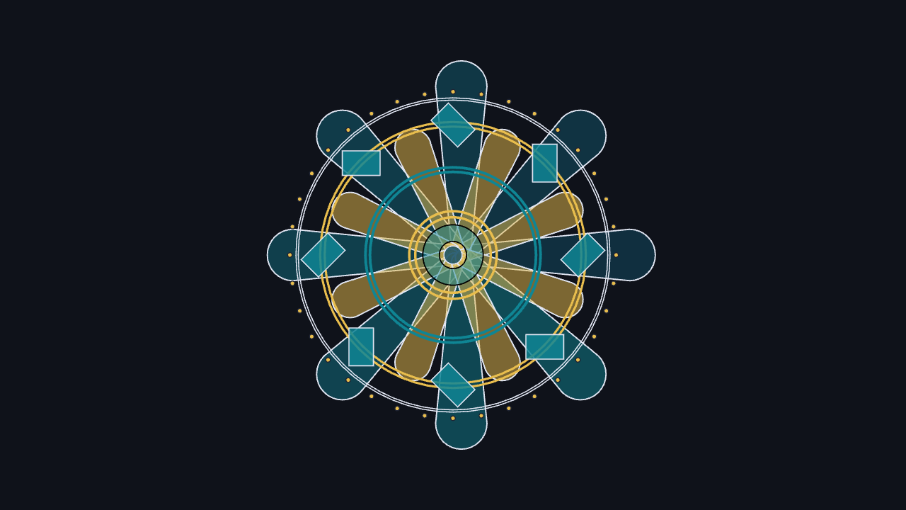
A still-image scene built from layered procedural petals, rings, and repeated geometric motifs.
# example: image render — no slides; export as a still image


background = [0.06, 0.07, 0.10, 1]
camera = Camera(6b)

let INK = [0.88, 0.9, 0.95, 1]
let DARK = [0.12, 0.14, 0.20, 1]
let DEEP = [0.07, 0.30, 0.39, 1]
let TEAL = [0.06, 0.52, 0.58, 1]
let BLUE = [0.33, 0.58, 0.88, 1]
let GOLD = [0.91, 0.74, 0.30, 1]

let petal_colors = [0.0 -> DEEP, 0.45 -> TEAL, 0.7 -> BLUE, 1.0 -> GOLD]

# custom operators keep repeated fill/stroke recipes concise
# they also allow for consistent
let glaze = operator |target, color_value, opacity = 0.6, width = 1.4|
    fill{alpha{opacity} color_value}
    stroke{INK, width}
    target

let trim = operator |target, color_value = GOLD, width = 2.2|
    fill{CLEAR}
    stroke{color_value, width}
    target

let Petal = |theta, radius, length, width, id| {
    # keyframe_lerp turns ring indices into a multi-stop radial color rhythm.
    let c = keyframe_lerp(petal_colors, id / 16)
    return tag{id}
        shift{[radius * cos(theta), radius * sin(theta), 0]}
        rotate{theta}
        glaze{c, 0.5, 1.1}
        Capsule([-length / 2, 0, 0], [length / 2, 0, 0], width)
}

let PetalRing = |count, radius, length, width, spin, base_id| block {
    # sample_clopen is almost useful here
    # but we need the index
    for (i in range(0, count)) {
        let theta = spin + i * TAU / count
        . Petal(theta, radius, length, width, base_id + i)
    }
}

let DotRing = |count, radius, dot_radius, color_value| block {
    for (i in range(0, count)) {
        let theta = i * TAU / count
        . fill{color_value}
          stroke{DARK, 0.8}
          shift{[radius * cos(theta), radius * sin(theta), 0]}
          Circle(dot_radius)
    }
}

let Diamond = |theta, radius, size, id| {
    let c = keyframe_lerp([0.0 -> GOLD, 0.4 -> BLUE, 1.0 -> TEAL], id / 8)
    return
        shift{[radius * cos(theta), radius * sin(theta), 0]}
        rotate{theta}
        glaze{c, 0.85, 0.9}
        rotate{TAU / 8}
        scale{[1.0, 0.65, 1]}
        Square(size)
}

let DiamondRing = |count, radius, size, spin, base_id| block {
    for (i in range(0, count)) {
        . Diamond(spin + i * TAU / count, radius, size, base_id + i)
    }
}

mesh core = [
    PetalRing(8, 1.22, 2.24, [0.12, 0.34], 0, 0),
    PetalRing(8, 0.88, 1.44, [0.12, 0.24], TAU / 16, 20)
]

mesh outline = [
    trim{TEAL, 2.2} Annulus(1.10, 1.16),
    trim{GOLD, 1.8} Annulus(1.70, 1.76),
    trim{INK, 0.9} Annulus(2.05, 2.08)
]

mesh accents = [
    DiamondRing(8, 1.72, 0.50, 0, 100),
    DotRing(36, 2.16, 0.03, GOLD)
]

mesh center = [
    fill{alpha{0.45} TEAL} Annulus(0.18, 0.40),
    trim{GOLD, 2.0} Annulus(0.50, 0.58),
    glaze{DEEP, 0.85, 0.9} Circle(0.12)
]A parameterized vector-field scene with arrows, streamlines, scripted changes, and an interactive pause.
# example: flow field / parameters
# If you enter presentation mode (Ctrl + P)
# and then toggle parameters (Ctrl + T),
# on the last slide, you will be able to edit parameters by hand
# and see the scene dynamically react!
let palette = [0 -> LIGHT_GRAY, 0.25 -> CYAN, 0.5 -> BLUE, 0.75 -> PURPLE, 1 -> RED]
let scene_scale = [2.35, 1.35, 1]
let bounds_x = [-2.75, 2.75]
let bounds_y = [-1.55, 1.55]
let soft = |col, amount| lerp(WHITE, col, amount)
let to_scene = |handle| [scene_scale[0] * handle[0], scene_scale[1] * handle[1], 0]
let safe_unit = |v| {
let n = norm(v)
if (n < 0.0001) { return 1r }
return v * (1 / n)
}
let flow_at = |pos, src, dst, swirl_value, pressure_value| {
# The field combines source/sink attraction with a tangential swirl term.
let src_delta = pos - src
let dst_delta = dst - pos
let src_d2 = max(0.12, dot(src_delta, src_delta))
let dst_d2 = max(0.12, dot(dst_delta, dst_delta))
let center_delta = pos - 0.5 * (src + dst)
let center_norm = max(0.35, norm(center_delta))
let tangent = [-center_delta[1], center_delta[0], 0] * (1 / center_norm)
let pressure_clamped = clamp(0.15, pressure_value, 1.8)
let swirl_clamped = clamp(-1.25, swirl_value, 1.25)
return pressure_clamped * (0.62 * src_delta * (1 / src_d2) + 0.82 * dst_delta * (1 / dst_d2)) +
0.42 * swirl_clamped * tangent
}
let Needle = |pos, src, dst, swirl_value, pressure_value, idx| {
let v = flow_at(pos, src, dst, swirl_value, pressure_value)
let strength = clamp(0, norm(v) / 3.2, 1)
let dir = safe_unit(v)
let len = 0.11 + 0.22 * strength
# keyframe_lerp is a compact way to turn many field samples into a gradient.
let col = keyframe_lerp(palette, strength)
return tag{[10, idx[0], idx[1]]}
color{col}
Arrow(pos - 0.5 * len * dir, pos + 0.5 * len * dir)
}
let NeedleField = |src, dst, swirl_value, pressure_value|
# Field handles the repeated sampling; Needle stays focused on one glyph.
Field(
|pos, idx| Needle(pos, src, dst, swirl_value, pressure_value, idx),
[bounds_x[0] + 0.24, bounds_x[1] - 0.24, 15],
[bounds_y[0] + 0.2, bounds_y[1] - 0.2, 9]
)
let streamline_points = |seed, src, dst, swirl_value, pressure_value| {
var points = []
var pos = seed
for (i in range(0, 42)) {
# A fixed Euler step keeps the path deterministic for animation replay.
points .= pos
pos = pos + 0.105 * safe_unit(flow_at(pos, src, dst, swirl_value, pressure_value))
}
return points
}
let Streamline = |seed, src, dst, swirl_value, pressure_value, id| {
let pts = streamline_points(seed, src, dst, swirl_value, pressure_value)
let col = keyframe_lerp(palette, id / 13)
return z_index{1}
tag{[100, id]}
stroke{soft(col, 0.55), 1.8}
Polyline(pts)
}
let Streamlines = |src, dst, swirl_value, pressure_value| block {
for (entry in enumerate(sample_clopen(0, TAU, 14))) {
let i = entry[0]
let theta = entry[1]
let seed = src + 0.18 * [cos(theta), sin(theta), 0]
. Streamline(seed, src, dst, swirl_value, pressure_value, i)
}
}
let Pole = |pos, color_value, sign, id| [
center{pos}
fill{soft(color_value, 0.18)}
stroke{color_value, 2.4}
Circle(0.2),
center{pos}
color{color_value}
Text(sign, 0.42),
center{pos}
fill{CLEAR}
stroke{soft(color_value, 0.45), 1.2}
Circle(0.38)
]
let FlowScene = |src, dst, swirl_value, pressure_value| {
let src_pos = to_scene(src)
let dst_pos = to_scene(dst)
return [
stroke{soft(LIGHT_GRAY, 0.24), 0.9}
LineGrid([bounds_x[0], bounds_x[1], 10], [bounds_y[0], bounds_y[1], 7], 1),
fill{CLEAR}
stroke{soft(LIGHT_GRAY, 0.55), 1.3}
Rect([bounds_x[1] - bounds_x[0], bounds_y[1] - bounds_y[0]]),
NeedleField(src_pos, dst_pos, swirl_value, pressure_value),
Streamlines(src_pos, dst_pos, swirl_value, pressure_value),
Pole(src_pos, ORANGE, "+", 200),
Pole(dst_pos, BLUE, "-", 210)
]
}
mesh field = FlowScene(
source: [-0.62, -0.22],
sink: [0.64, 0.34],
swirl: 0.38,
pressure: 0.9
)
"Scripted Change"
field.source = [-0.78, 0.42]
field.sink = [0.74, -0.35]
field.swirl = 0.95
field.pressure = 1.25
play Lerp(1.4)
play Wait(3)
field.source = [-0.42, 0.82]
field.sink = [0.28, -0.75]
field.swirl = -0.62
field.pressure = 0.45
play Lerp(1.4)
"Interactive Pause"
# here you can edit the parameters in presentation mode
# the true power of parameters
play Wait(2.0)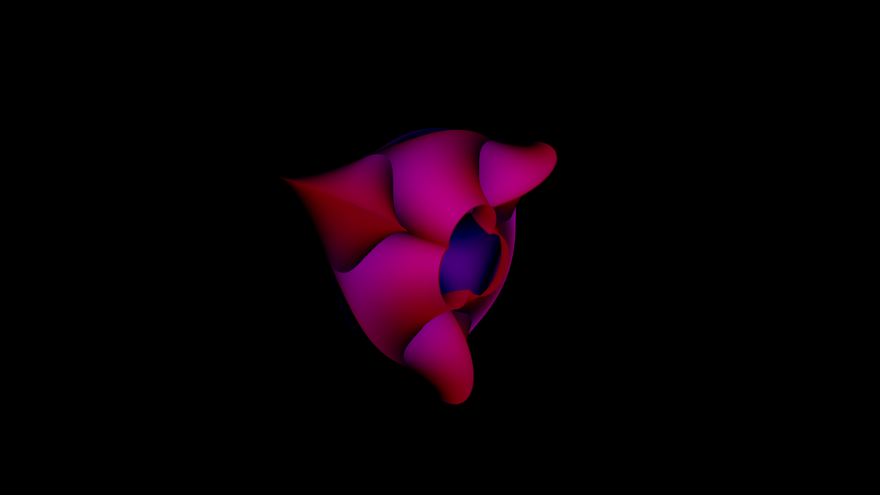
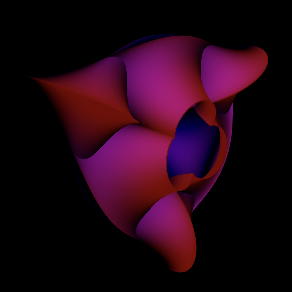
Monocurl logo
let u_samples = 128
let v_samples = 512

let Breather = |a, u_rad, v_rad| {
    let du = 2 * u_rad / u_samples
    let dv = 2 * v_rad / v_samples

    let f = |u, v| {
        let wsqr = 1 - a * a
        let w = sqrt(wsqr)
        let denom = a * ((w * cosh(a * u)) ^ 2 + (a * sin(w * v)) ^ 2)

        let x = -u + (2 * wsqr * cosh(a * u) * sinh(a * u) / denom)
        let y = 2 * w * cosh(a * u) * (-(w * cos(v) * cos(w * v)) - (sin(v) * sin(w * v))) / denom
        let z = 2 * w * cosh(a * u) * (-(w * sin(v) * cos(w * v)) + (cos(v) * sin(w * v))) / denom

        return [-x, y, z]
    }

    return (
        gloss{0.5}
        color_map{|x| f(1.5 * x[0], x[0]) .. 1}
        point_map{|x| f(x[0], x[1])}
            ColorGrid(
                |_, _| RED,
                [-u_rad, u_rad, u_samples],
                [-v_rad, v_rad, v_samples]
           )
    )
}

let a = 0.8
mesh logo = Breather(a, 3, TAU * 4 / 3 / a)

background = BLACK
camera = Camera(position: [-4, 2, -4])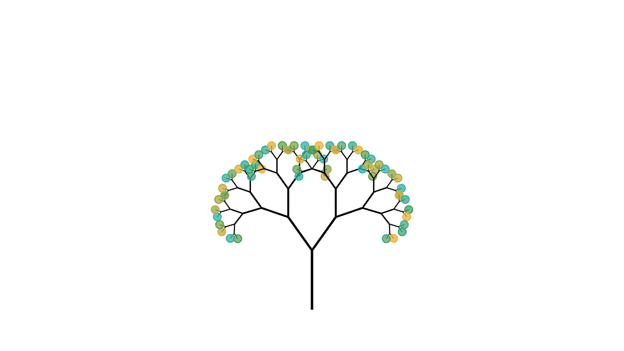
A recursive mesh image where one branch returns two smaller branches with stable structure and colored leaves.
# example: fractals / recursive meshes
camera = Camera(5b)
let rot = |v, angle| [
cos(angle) * v[0] - sin(angle) * v[1],
sin(angle) * v[0] + cos(angle) * v[1],
0
]
let leaf_colors = [0 -> TEAL, 0.45 -> GREEN, 1 -> ORANGE]
# notice that recursive functions take themselves as parameters
# this is familiar if you've seen untyped lambda calculus
let Branch = |self, depth, at, dir, length, angle, shrink, id| {
if (depth <= 0) {
let hue = keyframe_lerp(leaf_colors, (sin(id) + 1) / 2)
return
fill{alpha{0.5} hue}
stroke{hue, 1.2}
center{at}
Circle(0.06 + 0.045 * length)
}
let end = at + length * dir
let stroke_width = 0.6 + depth * 0.34
return [
stroke{BLACK, stroke_width} Line(at, end),
# recursive calls
self(self, depth - 1, end, rot(dir, angle), length * shrink, angle, shrink, 2 * id),
self(self, depth - 1, end, rot(dir, -angle), length * shrink, angle, shrink, 2 * id + 1)
]
}
let RecursiveTree = |depth, angle, shrink|
Branch(Branch, to_int(depth), [0, -2.15, 0], UP, 0.95, angle, shrink, 1)
"Recursive Tree"
mesh tree = RecursiveTree(depth: 7, angle: 0.62, shrink: 0.69)
play Set()A 3D camera animation scene that introduces Monocurl's rendered animation workflow.
# example: 3d camera animation
let samples = 24
let height = |x, y| 1.15 * ((x - 0.5) ^ 2 + (y - 0.5) ^ 2)
let color_keys = [0 -> BLUE, 0.15 -> YELLOW, 0.3 -> ORANGE, 0.55 -> RED]
let color_at = |pos, idx| {
let value = height(pos[0], -pos[1])
# keyframe_lerp turns a scalar field into a smooth multi-stop surface gradient.
return keyframe_lerp(color_keys, value)
}
"Flat Grid"
mesh grid = stroke{BLACK, 1.5} ColorGrid(
|pos, idx| BLACK,
[0, 1, samples],
[-1, 0, samples]
)
mesh axis =
shift{[0, 0, -0.01]} # draw below function
axis_style{"x", 0, 1, "x"}
axis_style{"y", 0, 1, "y"}
axis_style{"z", 0, 1, "z"}
Axis3d(
basis: [1r, 1d, 1b],
color: BLACK,
grid_color: LIGHT_GRAY,
[1u, 1u, 1b]
)
mesh monocurl = center{0.7u} Text("Monocurl", 2)
play [Fade(0.8, [&axis, &grid]), Write(0.8, &monocurl)]
"Surface And Camera"
# an anim block is analogous to a coroutine in other languages
# it does nothing until it is played
let lift_grid = anim {
grid = stroke{BLACK, 1.5} ColorGrid(
color_at,
[0, 1, samples],
[-1, 0, samples]
)
play Trans(0.8, [&grid])
grid =
point_map{|point| [point[0], point[1], height(point[0], point[1] + 1)]}
grid
play Trans(1.8, [&grid])
}
# CameraLerp interpolates camera movement more smoothly than a plain Lerp.
let move_camera = anim {
camera = Camera([2.2, -2.1, 1.45], [0.5, -0.5, 0.35], [0, 0, 1])
play CameraLerp(&camera, 2.6)
}
play [lift_grid, move_camera]
play Wait(0.4)A line-by-line inequality transformation showing tagged LaTeX expressions and topology-aware text morphs.
# example: am-gm inequality
"AM-GM Inequality"
# This shows how you can transform between succesive inequalities
# line-by-line
#
# It's admittedly more tedious than other animation libraries
# but the upside is this is not special cased into the stdlib
# (allowing greater generality)
#
# LLM's can also be helpful in removing some of the tediousness
#
# Eventually, this may be more automated in a library
# to support the common operations/behavior at least
# instead of having to repeatedly type tags
# you can save the entire value as a constant and reference that
let x = text_tag{1} "x"
let a = text_tag{1} "a"
let x2 = text_tag{2} "x^2"
let ap = text_tag{2} "a"
let y = text_tag{3} "y"
let b = text_tag{3} "b"
let y2 = text_tag{4} "y^2"
let bp = text_tag{4} "b"
let ge = "\ \tag9{\ge} \ "
let palette = operator |target|
color{ORANGE, |tag| 3 in tag or 4 in tag}
color{BLUE, |tag| 1 in tag or 2 in tag}
target
# while it is possible to use latex align* for this purpose
# it's slightly harder to recover
# what "row/equation" each mesh came from, making the animations
# more difficult
# (With align*, it would be done via preprocessing each element with an additional tag component to keep row information)
# make untagged portions fade in and out by giving them
# row-unique tag
let retag_empty = operator |operand, new|
tag_map{|old, leaf| {
if (old == []) { return tag{new} leaf }
return leaf
}} operand
let Inequality = |lhs, rhs, row_id| {
print to_string(lhs)
let latex = Tex([lhs, ge, rhs])
let ge = tag_filter{|tag| 9 in tag} latex
let pos = mesh_center(ge)
return retag_empty{-row_id - 100} shift{[1-pos[0], 0, 0]} palette{} latex
}
let AlignedInequalities = |equations| {
return shift{1.5u} Stack(equations, 1d)
}
let PushEquation = |&container, lhs, rhs, tag_map=nil| anim {
let ie = Inequality(lhs, rhs, len(container.rows))
if (container.rows == []) {
container.rows .= ie
play Write(1)
}
else {
# strategy: compute the full mesh and extract
# out the last two rows
# create an auxiliary mesh that transforms from second
# to last row to the last row
# then delete auxiliary and show full unmodified container
container.rows .= ie
# by accessing container[i] instead of container.rows[i]
# we access the SHIFTED / positioned mesh
# which is what we want
let count = len(container.rows)
mesh tmp = container[count - 2]
play Set(&tmp)
tmp = container[count - 1]
play set_default{"tag_map", tag_map} TagTrans(1, &tmp)
tmp = []
play Set()
}
play Wait(1)
}
mesh curr = AlignedInequalities(rows: [])
# https://www.cantorsparadise.com/an-introduction-to-the-am-gm-inequality-38f7895e8f30
play PushEquation(&curr,
["(", x, "-", y, ")^2"],
["\tag8{0}"]
)
play PushEquation(&curr,
[x2, "-\tag7{2}", x, y, "+", y2],
["\tag8{0}"],
# x becomes x and x^2 in next line
[[1]->[[1], [2]],
[3]->[[3], [4]]]
)
play PushEquation(&curr,
[x2, "+", y2],
["\tag7{2}", x, y]
)
play PushEquation(&curr,
["\frac{", x2, "+", y2, "}{", "\tag7{2}", "}"],
[x, y]
)
play PushEquation(&curr,
["\text{Letting $",ap,"=",x2,"$ and $",bp,"=",y2,"$ \quad}",
"\frac{", ap, "+", bp, "}{", "\tag7{2}", "}"],
["\sqrt{", a, b, "}"]
)