
Monocurl Essays
Series Download

Roots, factors and the shape of a polynomial

A cubic crosses the x axis once or three times, never exactly twice. The factor theorem, multiplicity and the leading term explain why, with proofs.

23 min·High school·

AssumesThe distributive law as a picture: FOIL and (a+b)²Shifting and stretching graphs: why f(x - 2) moves right

The graph of $y = x^3 - 3x + c$ as $c$ falls from 4 to 0, which lowers the whole curve. It crosses the $x$ axis once, then touches it at a second point when $c = 2$, and after that crosses three times. At no stage are there exactly two crossings.
Monocurl source
let fh = Frame(-3, 3, -6, 8, [-0.95, 0.05, 0], 4.8, 3.5)
let Lift = |c| {
    let pts = filter(map(sample(-3, 3, 240), |x| [x, x * x * x - 3 * x + c]), |q| q[1] > -6 and q[1] < 8)
    var out = [stroke{AZURE, 4.5} Polyline(map(pts, |q| at(fh, q[0], q[1])))]
    var count = 0
    for (j in range(0, len(pts) - 1)) {
        let a = pts[j]
        let b = pts[j + 1]
        if ((a[1] < 0) != (b[1] < 0)) {
            count = count + 1
            out .= Pt(at(fh, a[0] - a[1] * (b[0] - a[0]) / (b[1] - a[1]), 0), LEAF, 0.11)
        }
    }
    if (abs(c - 2) < 0.03) {
        out .= Ring(at(fh, 1, 0), ROSE, 0.14, 3.5)
        out .= center{at(fh, 1, -1.4)} Cap("touches", 0.74, ROSE)
    }
    out .= center{[3.2, 0.75, 0]} scale{1.1} color{INK} Number(c, 2)
    out .= center{[2.9, -0.85, 0]} scale{1.8} color{LEAF} Number(count, 0)
    return out
}
mesh plot = Plot(fh, [-3, -2, -1, 0, 1, 2, 3], [-6, -4, -2, 2, 4, 6, 8])
mesh labels = [
    center{[2.9, 1.5, 0]} Math("y = x^3 - 3x + c", 0.8, AZURE),
    center{[2.5, 0.75, 0]} Math("c =", 0.9, INK),
    center{[2.9, -0.2, 0]} Note("crossings", 0.76)
]
mesh lift = Lift(c: 4)

slide "lower"
    play Wait(1)
    lift.c = 2
    play Lerp(2.5, [&lift])
    play Wait(1.5)
    lift.c = 0
    play Lerp(2.5, [&lift])
    play Wait(2)

Uses the shared definitions for this lesson's figures.

Draw the graph of a cubic, any cubic, and count how many times it crosses the $x$ axis. You will get one or three. Slide the graph up and down, as in the animation, and the count changes from one to three by passing through a moment when the curve touches the axis without crossing it. A count of exactly two clean crossings never appears. Parabolas have their own rule: zero or two.

Nothing about the look of the formula $x^3 - 3x + c$ announces this. The explanation has three parts, and each is a theorem about polynomials in general: a root of a polynomial is the same thing as a factor of it; the far ends of the graph are decided by one term; and whether the graph crosses or touches at a root is decided by how many times the factor occurs. We will prove all three.

A polynomial and its roots

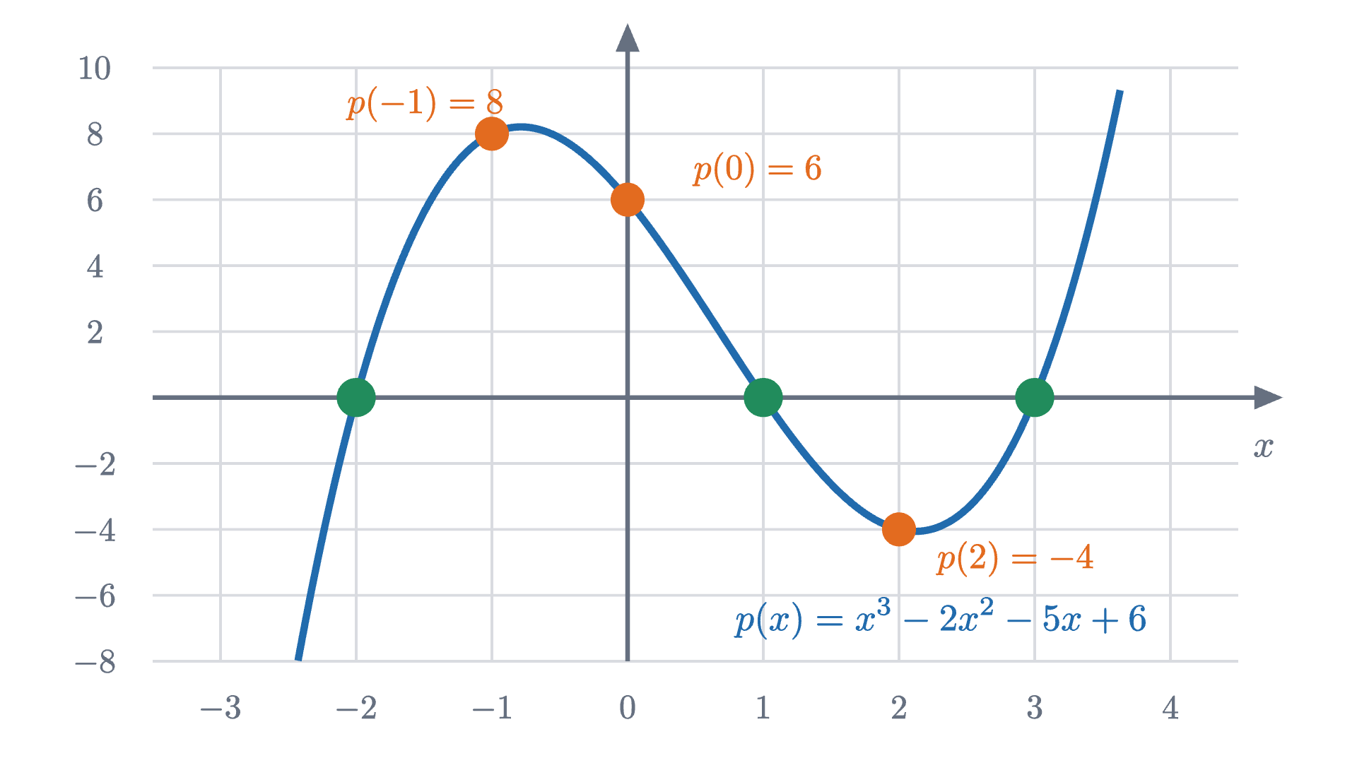
On the graph, the real roots are the places where the curve meets the $x$ axis. Our running example is the cubic
$$ p(x) = x^3 - 2x^2 - 5x + 6. $$
The graph of p(x) = x^3 - 2x^2 - 5x + 6, with its value marked at each whole number from -2 to 3. The value is 0 at x = -2, x = 1 and x = 3 (green), and those are the three roots.
The graph of $p(x) = x^3 - 2x^2 - 5x + 6$, with its value marked at each whole number from $-2$ to 3. The value is 0 at $x = -2$, $x = 1$ and $x = 3$ (green), and those are the three roots.
Monocurl source
let fp = Frame(-3.5, 4.5, -8, 10, [0.1, 0.1, 0], 6.4, 3.5)
mesh plot = Plot(fp, [-3, -2, -1, 0, 1, 2, 3, 4], [-8, -6, -4, -2, 2, 4, 6, 8, 10])
mesh curve = Curve(fp, pv, -3.5, 4.5)
mesh dots = block {
    for (a in [-1, 0, 2]) {
        . Pt(at(fp, a, pv(a)), EMBER, 0.095)
    }
    for (a in [-2, 1, 3]) {
        . Pt(at(fp, a, 0), LEAF, 0.11)
    }
}
mesh names = [
    center{at(fp, -1.5, 8.9)} Math("p(-1) = 8", 0.76, EMBER),
    center{at(fp, 0.95, 6.9)} Math("p(0) = 6", 0.76, EMBER),
    center{at(fp, 2.85, -4.9)} Math("p(2) = -4", 0.76, EMBER),
    center{at(fp, 2.3, -6.7)} Math("p(x) = x^3 - 2x^2 - 5x + 6", 0.8, AZURE)
]

Uses the shared definitions for this lesson's figures.

Finding the roots $-2$, 1 and 3 took nothing more than trying whole numbers. The interesting question is what a root tells us about the formula. The same thing happens with whole numbers: 7 goes into 91 exactly, and knowing that lets us write $91 = 7 \times 13$. To see whether a root does something similar we divide $p(x)$ by an expression of the form $x - a$, and it is instructive to begin with an $a$ that is not a root, $a = 2$.

Dividing polynomials works like long division of numbers: at each stage, match the leading term of what is left.

  1. Match the leading term first. To get x cubed from x - 2 we need to multiply by x squared, and x squared times (x - 2) is x cubed minus 2 x squared. That accounts for the first two terms.
  2. What is left is -5x + 6. Match its leading term: -5 times (x - 2) is -5x + 10, which is 4 too many, so the last piece is -4.
  3. Collect the two multiples of x - 2. The quotient is x squared minus 5, and the remainder is -4.
  4. Now put x = 2 into the last line. The first part becomes zero, so p(2) equals the remainder.
Dividing $p(x) = x^3 - 2x^2 - 5x + 6$ by $x - 2$. At each stage a multiple of $x - 2$ is split off that accounts for the leading term of what remains.
Monocurl source
let Line = |k, parts| center{[0, 1.75 - 0.88 * k, 0]} color{ROSE, |tags| 2 in tags} color{AZURE, |tags| 1 in tags} color{INK} Tex(parts, 1.3)
mesh lines = [Line(0, ["p(x) = x^3 - 2x^2 - 5x + 6"])]

slide "Match the leading term first. To get x cubed from x - 2 we need to multiply by x squared, and x squared times (x - 2) is x cubed minus 2 x squared. That accounts for the first two terms."
    lines .= Line(1, ["= ", text_tag{1} "(x - 2)\,x^2", "\; + \;", text_tag{2} "(-5x + 6)"])
    play Fade(0.7, [&lines])

slide "What is left is -5x + 6. Match its leading term: -5 times (x - 2) is -5x + 10, which is 4 too many, so the last piece is -4."
    lines .= Line(2, ["= ", text_tag{1} "(x - 2)\,x^2 + (x - 2)(-5)", "\; + \;", text_tag{2} "(-4)"])
    play Fade(0.7, [&lines])

slide "Collect the two multiples of x - 2. The quotient is x squared minus 5, and the remainder is -4."
    lines .= Line(3, ["= ", text_tag{1} "(x - 2)(x^2 - 5)", "\; + \;", text_tag{2} "(-4)"])
    play Fade(0.7, [&lines])

slide "Now put x = 2 into the last line. The first part becomes zero, so p(2) equals the remainder."
    lines .= Line(4, ["p(2) = ", text_tag{1} "0 \cdot (2^2 - 5)", "\; + \;", text_tag{2} "(-4)", " = -4"])
    play Fade(0.7, [&lines])

Uses the shared definitions for this lesson's figures.

The result is $p(x) = (x - 2)(x^2 - 5) - 4$: a quotient $x^2 - 5$ and a remainder $-4$, which is a constant. And the remainder $-4$ is the number we met in the graph as $p(2)$.

Pause and try

Divide $p(x) = x^3 - 2x^2 - 5x + 6$ by $x - 1$ in the same way. What are the quotient and the remainder? Then predict, without dividing, the remainder when $p(x)$ is divided by $x + 1$.

Show answerHide answer

First $x^2(x - 1) = x^3 - x^2$, leaving $-x^2 - 5x + 6$. Then $-x(x - 1) = -x^2 + x$, leaving $-6x + 6$. Then $-6(x - 1) = -6x + 6$, leaving 0. So $p(x) = (x - 1)(x^2 - x - 6)$, with remainder 0. For the prediction, note that $x + 1 = x - (-1)$. If the pattern holds, the remainder is $p(-1) = 8$, and it is: $p(x) = (x + 1)(x^2 - 3x - 2) + 8$.

Here $a$ slides along the axis while the division is redone at every position.

Dividing $p(x)$ by $x - a$ as $a$ moves from $-2.4$ to 3, pausing at the three roots. The remainder always equals the height $p(a)$ of the graph above $a$, so it is 0 exactly when $a$ is a root.
Monocurl source
let fd = Frame(-3.5, 4.5, -8, 10, [-1.05, 0.1, 0], 4.6, 3.5)
let Div = |a| {
    let b = a - 2
    let cc = a * b - 5
    let r = a * cc + 6
    return [
        Seg(at(fd, a, 0), at(fd, a, pv(a)), EMBER, 4),
        Pt(at(fd, a, 0), EMBER, 0.08),
        Pt(at(fd, a, pv(a)), EMBER, 0.1),
        center{[3.1, 1.3, 0]} scale{1.1} color{EMBER} Number(nz(a), 2),
        center{[2.45, 0.15, 0]} scale{0.9} color{AZURE} Number(nz(b), 1, 1),
        center{[3.5, 0.15, 0]} scale{0.9} color{AZURE} Number(nz(cc), 1, 1),
        center{[2.75, -0.95, 0]} scale{1.25} color{ROSE} Number(nz(r), 2),
        center{[2.75, -1.92, 0]} scale{1.25} color{EMBER} Number(nz(pv(a)), 2)
    ]
}
mesh plot = Plot(fd, [-3, -2, -1, 0, 1, 2, 3, 4], [-8, -4, 4, 8])
mesh curve = Curve(fd, pv, -3.5, 4.5)
mesh labels = [
    center{[2.75, 1.82, 0]} Math("\text{divide by } x - a", 0.8, SLATE),
    center{[2.35, 1.3, 0]} Math("a =", 0.9, EMBER),
    center{[2.75, 0.62, 0]} Note("quotient", 0.74),
    center{[1.85, 0.15, 0]} Math("x^2", 0.85, AZURE),
    center{[2.98, 0.15, 0]} Math("x", 0.85, AZURE),
    center{[2.75, -0.48, 0]} Note("remainder", 0.74),
    center{[2.75, -1.45, 0]} Note("height of graph, p(a)", 0.74)
]
mesh div = Div(a: -2.4)

slide "slide"
    play Wait(0.5)
    div.a = -2
    play Lerp(1, [&div])
    play Wait(1)
    div.a = 1
    play Lerp(3, [&div])
    play Wait(1)
    div.a = 3
    play Lerp(2.5, [&div])
    play Wait(1.8)

Uses the shared definitions for this lesson's figures.

Why the remainder is p(a): the factor theorem

The last step of the division figure already contains the reason. If $p(x) = (x - a)\,q(x) + r$ with $r$ a constant, then putting $x = a$ makes the first part vanish and leaves $p(a) = r$. What still needs proof is that such a quotient $q$ and constant $r$ always exist. Long division produces them in every example, but “it always works” is a claim about all polynomials, and there is a short argument that covers them all at once. It rests on one identity.

For every whole number $k \ge 1$,

$$ x^k - a^k = (x - a)\left(x^{k-1} + a\,x^{k-2} + a^2x^{k-3} + \cdots + a^{k-1}\right). $$

To check it, multiply the long bracket by $x$ and by $a$ separately. Multiplying by $x$ gives $x^k + a\,x^{k-1} + \cdots + a^{k-1}x$. Multiplying by $a$ gives $a\,x^{k-1} + \cdots + a^{k-1}x + a^k$. Subtracting, every term cancels except $x^k$ and $a^k$. (This is the finite sum formula of the lesson on geometric series in other clothes. For $k = 2$ it is $x^2 - a^2 = (x - a)(x + a)$.)

Check the proof against the example with $a = 2$: $p(x) - p(2) = (x^3 - 8) - 2(x^2 - 4) - 5(x - 2) = (x - 2)\left[(x^2 + 2x + 4) - 2(x + 2) - 5\right] = (x - 2)(x^2 - 5)$, the quotient that long division found. The proof used only addition and multiplication, so it holds equally when the coefficients and $a$ are complex numbers.

How many roots can there be?

Apply the factor theorem to our cubic. Since $p(1) = 0$, we get $p(x) = (x - 1)(x^2 - x - 6)$, as you found by dividing. The quotient has roots of its own: $x^2 - x - 6$ vanishes at $x = -2$, so it equals $(x + 2)(x - 3)$. Altogether

$$ p(x) = (x - 1)(x + 2)(x - 3). $$

Each root has been turned into a factor, and each factor has used up one unit of degree.

  1. The cubic p has degree 3 and three roots.
  2. Divide out the factor x - 1. The quotient is a parabola. It no longer vanishes at 1, and it still has the other two roots, -2 and 3.
  3. Divide the parabola by x + 2. The quotient is the line x - 3, with the single root 3.
  4. Divide the line by x - 3. The quotient is the constant 1. A nonzero constant has no roots, so there cannot be a fourth root.
Each root of the cubic $p$ is divided out in turn. The quotient loses one degree and one root each time, and after three divisions nothing is left but the constant 1, which has no roots.
Monocurl source
let fe = Frame(-3.5, 4.5, -8, 10, [-1.05, 0.1, 0], 4.6, 3.5)
let quad = |x| x * x - x - 6
let lin = |x| x - 3
let one = |x| 1
let Roots = |live, dead| block {
    for (a in dead) {
        . Ring(at(fe, a, 0), SLATE, 0.1, 3)
    }
    for (a in live) {
        . Pt(at(fe, a, 0), LEAF, 0.11)
    }
}
let Side = |top, formula, size, col, deg, rts| [
    center{[2.75, 1.5, 0]} Math(top, 1.05, SLATE),
    center{[2.75, 0.6, 0]} Math(formula, size, col),
    center{[2.75, -0.35, 0]} Math(deg, 0.95, SLATE),
    center{[2.75, -1.15, 0]} Math(rts, 0.95, LEAF)
]
mesh plot = Plot(fe, [-3, -2, -1, 0, 1, 2, 3, 4], [-8, -4, 4, 8])
mesh old = []
mesh cur = Curve(fe, pv, -3.5, 4.5, AZURE)
mesh roots = Roots([-2, 1, 3], [])
mesh side = Side("p(x)", "x^3 - 2x^2 - 5x + 6", 0.8, AZURE, "\text{degree } 3", "\text{roots } -2,\ 1,\ 3")

slide "The cubic p has degree 3 and three roots."
    play Wait(0.5)

slide "Divide out the factor x - 1. The quotient is a parabola. It no longer vanishes at 1, and it still has the other two roots, -2 and 3."
    side = []
    play Fade(0.3, [&side])
    old .= Curve(fe, pv, -3.5, 4.5, tint(AZURE, 0.35), 3)
    cur = Curve(fe, quad, -3.5, 4.5, EMBER)
    roots = Roots([-2, 3], [1])
    side = Side("\div\ (x - 1)", "x^2 - x - 6", 1.05, EMBER, "\text{degree } 2", "\text{roots } -2,\ 3")
    play Fade(0.8)

slide "Divide the parabola by x + 2. The quotient is the line x - 3, with the single root 3."
    side = []
    play Fade(0.3, [&side])
    old .= Curve(fe, quad, -3.5, 4.5, tint(EMBER, 0.35), 3)
    cur = Curve(fe, lin, -3.5, 4.5, PLUM)
    roots = Roots([3], [1, -2])
    side = Side("\div\ (x + 2)", "x - 3", 1.15, PLUM, "\text{degree } 1", "\text{root } 3")
    play Fade(0.8)

slide "Divide the line by x - 3. The quotient is the constant 1. A nonzero constant has no roots, so there cannot be a fourth root."
    side = []
    play Fade(0.3, [&side])
    old .= Curve(fe, lin, -3.5, 4.5, tint(PLUM, 0.35), 3)
    cur = stroke{GOLD, 4} Line(at(fe, -3.5, 1), at(fe, 4.5, 1))
    roots = Roots([], [1, -2, 3])
    side = Side("\div\ (x - 3)", "1", 1.3, GOLD, "\text{degree } 0", "\text{no roots}")
    play Fade(0.8)

Uses the shared definitions for this lesson's figures.

The hypothesis hidden in the word “degree” matters. The zero polynomial, all of whose coefficients are 0, has no degree, and every number is a root of it.

So a cubic has at most three roots and a quadratic at most two. It is tempting to go further and say a polynomial of degree $n$ has exactly $n$ roots. That is false for real roots: $x^2 + 1$ has none, and the cubic $x^3 - 3x + 4$ at the start of the hero animation has one. The missing roots exist, but they are complex numbers. This is the fundamental theorem of algebra: every polynomial of degree at least 1, with real or complex coefficients, has at least one complex root. It was proved in the early nineteenth century (Gauss and Argand gave the first proofs that were widely accepted), every known proof uses some fact about continuity or the real numbers that goes beyond algebra, and we cite it without proof. Combined with the factor theorem, used once per root as in the figure above, it implies that a polynomial of degree $n$ factors completely as $c\,(x - z_1)(x - z_2)\cdots(x - z_n)$ with complex $z_1, \ldots, z_n$, some of which may be equal.

The three complex roots of $x^3 - 3x + c$ as $c$ rises from 0 to 12. At first all three lie on the real axis (green). At $c = 2$ two of them collide at $x = 1$, and for larger $c$ they leave the real axis as a pair of mirror images (purple). There are always three.
Monocurl source
let cpt = |o, u, z| [o[0] + u * z[0], o[1] + u * z[1], 0]
let O7 = [-0.6, 0, 0]
let U7 = 0.9
let plane = block {
    for (x in range(-3, 3)) {
        . Seg(cpt(O7, U7, [x, -2]), cpt(O7, U7, [x, 2]), MIST, 1.5)
        . center{[O7[0] + U7 * x, O7[1] - 2 * U7 - 0.27, 0]} Math(to_string(x), 0.72, SLATE)
    }
    for (y in range(-2, 3)) {
        . Seg(cpt(O7, U7, [-3, y]), cpt(O7, U7, [2, y]), MIST, 1.5)
    }
    . center{[O7[0] - 3 * U7 - 0.36, O7[1] + 2 * U7, 0]} Math("2i", 0.72, SLATE)
    . center{[O7[0] - 3 * U7 - 0.36, O7[1] + U7, 0]} Math("i", 0.72, SLATE)
    . center{[O7[0] - 3 * U7 - 0.36, O7[1] - U7, 0]} Math("-i", 0.72, SLATE)
    . center{[O7[0] - 3 * U7 - 0.36, O7[1] - 2 * U7, 0]} Math("-2i", 0.72, SLATE)
    . Tip(cpt(O7, U7, [-3, 0]), [O7[0] + 2 * U7 + 0.28, O7[1], 0], SLATE, 2.5, 0.15)
    . Tip(cpt(O7, U7, [0, -2]), [O7[0], O7[1] + 2 * U7 + 0.28, 0], SLATE, 2.5, 0.15)
    . center{[O7[0] + 2 * U7 - 0.22, O7[1] - 0.26, 0]} Note("real", 0.72)
    . center{[O7[0] + 0.85, O7[1] + 2 * U7 + 0.2, 0]} Note("imaginary", 0.72)
}
let Roots = |c| {
    # the leftmost root is always real; find it by bisection, then solve the quadratic that is left
    var lo = -3.2
    var hi = -1.7
    for (j in range(0, 40)) {
        let mid = (lo + hi) / 2
        if (mid * mid * mid - 3 * mid + c < 0) {
            lo = mid
        } else {
            hi = mid
        }
    }
    let r = (lo + hi) / 2
    let disc = 12 - 3 * r * r
    var out = [Pt(cpt(O7, U7, [r, 0]), LEAF, 0.12)]
    var reals = 1
    if (disc >= 0) {
        reals = 3
        out .= Pt(cpt(O7, U7, [(-r - sqrt(disc)) / 2, 0]), LEAF, 0.12)
        out .= Pt(cpt(O7, U7, [(-r + sqrt(disc)) / 2, 0]), LEAF, 0.12)
    } else {
        out .= Pt(cpt(O7, U7, [-r / 2, sqrt(-disc) / 2]), PLUM, 0.12)
        out .= Pt(cpt(O7, U7, [-r / 2, -sqrt(-disc) / 2]), PLUM, 0.12)
    }
    out .= center{[3.0, 0.85, 0]} scale{1.1} color{INK} Number(c, 2)
    out .= center{[2.7, -0.2, 0]} scale{1.4} color{LEAF} Number(reals, 0)
    out .= center{[2.7, -1.4, 0]} scale{1.4} color{PLUM} Number(3 - reals, 0)
    return out
}
mesh grid = plane
mesh labels = [
    center{[2.7, 1.55, 0]} Math("x^3 - 3x + c = 0", 0.8, INK),
    center{[2.3, 0.85, 0]} Math("c =", 0.9, INK),
    center{[2.7, 0.3, 0]} Note("real roots", 0.74),
    center{[2.7, -0.9, 0]} Note("non-real roots", 0.74)
]
mesh roots = Roots(c: 0)

slide "roots"
    play Wait(0.8)
    roots.c = 2
    play Lerp(2.5, [&roots])
    play Wait(1.2)
    roots.c = 12
    play Lerp(3.5, [&roots])
    play Wait(1.8)

Uses the shared definitions for this lesson's figures.

Crossing or touching: multiplicity

At $c = 2$ the hero cubic is $x^3 - 3x + 2$, which factors as $(x - 1)^2(x + 2)$. The factor $x - 1$ occurs twice, and $x = 1$ is where the graph touches the axis and turns back.

Every root of a polynomial of degree $n$ has a multiplicity between 1 and $n$. Divide by $x - a$ for as long as the quotient still vanishes at $a$; each division lowers the degree by one, so this stops after at most $n$ divisions, at a quotient $q$ with $q(a) \ne 0$.

Pause and try

Let $h(x) = \frac14(x + 2)(x - 1)^2(x - 3)$. Work out the sign of each of the factors $x + 2$, $(x - 1)^2$ and $x - 3$ just to the left and just to the right of each root, and from them the sign of $h$. At which roots does the graph cross the axis?

Show answerHide answer

Near $x = -2$: $(x - 1)^2 > 0$ and $x - 3 < 0$ on both sides, while $x + 2$ changes from negative to positive. So $h$ changes from positive to negative: a crossing. Near $x = 1$: $x + 2 > 0$ and $x - 3 < 0$ on both sides, and $(x - 1)^2$ is positive on both sides. So $h$ is negative on both sides and zero at 1: the graph touches the axis from below. Near $x = 3$: only $x - 3$ changes sign, so $h$ changes from negative to positive: a crossing.
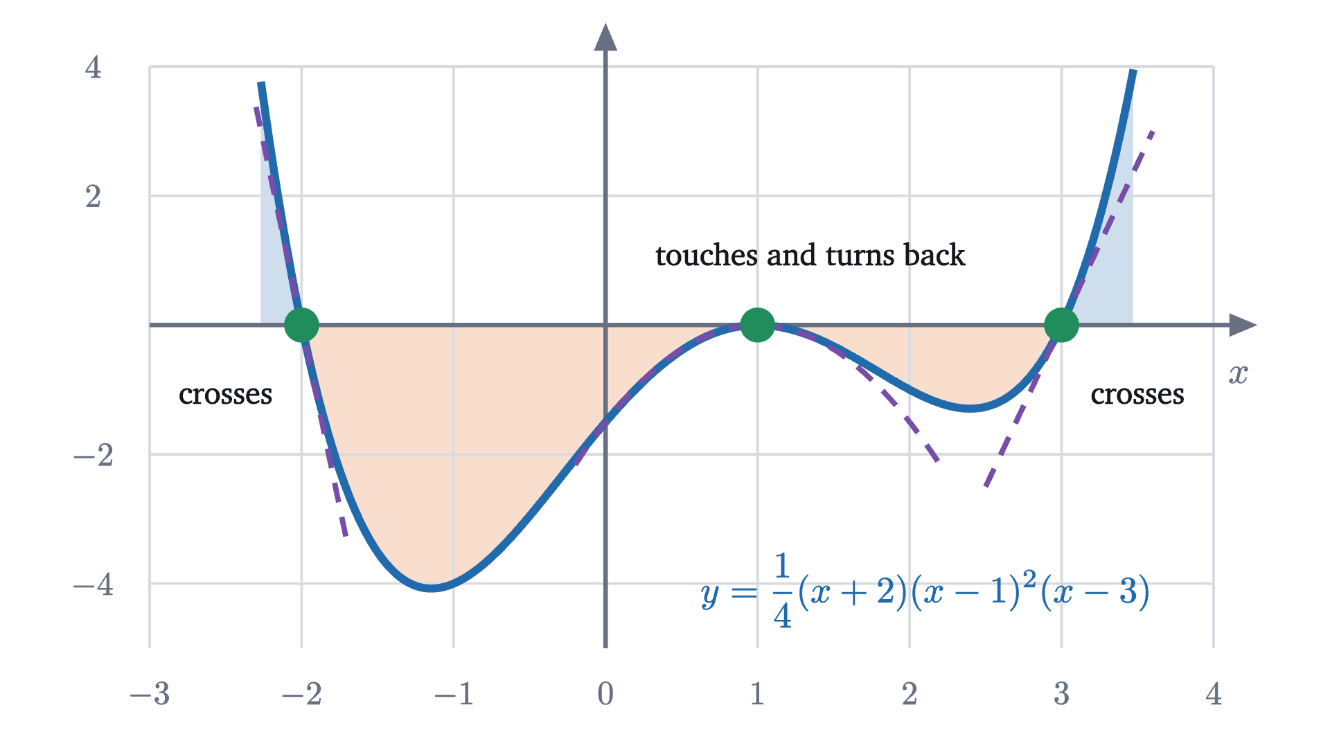
The graph of h(x) = \frac14(x + 2)(x - 1)^2(x - 3), shaded where it is positive (blue) and negative (orange). Near each root it follows the dashed curve obtained by freezing the other factors at their values there: a line at the simple roots -2 and 3, and a parabola at the double root 1.
The graph of $h(x) = \frac14(x + 2)(x - 1)^2(x - 3)$, shaded where it is positive (blue) and negative (orange). Near each root it follows the dashed curve obtained by freezing the other factors at their values there: a line at the simple roots $-2$ and 3, and a parabola at the double root 1.
Monocurl source
let fm = Frame(-3, 4, -5, 4, [0.1, 0.1, 0], 6.4, 3.5)
let hv = |x| (x + 2) * (x - 1) * (x - 1) * (x - 3) / 4
let Shade = |a, b, col| Region(
    flatten([[at(fm, a, 0)], map(sample(a, b, 60), |x| at(fm, x, clamp(-5, hv(x), 4))), [at(fm, b, 0)]]),
    tint(col, 0.22)
)
let Local = |f, a, b| stroke{PLUM, 3} dashed{[0.12, 0.09]} Polyline(map(sample(a, b, 40), |x| at(fm, x, f(x))))
mesh shades = [
    Shade(-2.27, -2, AZURE),
    Shade(-2, 1, EMBER),
    Shade(1, 3, EMBER),
    Shade(3, 3.47, AZURE)
]
mesh plot = Plot(fm, [-3, -2, -1, 0, 1, 2, 3, 4], [-4, -2, 2, 4])
mesh curve = Curve(fm, hv, -3, 4, AZURE, 4.5)
mesh locals = [
    Local(|x| -11.25 * (x + 2), -2.3, -1.7),
    Local(|x| -1.5 * (x - 1) * (x - 1), -0.2, 2.2),
    Local(|x| 5 * (x - 3), 2.5, 3.6)
]
mesh dots = [Pt(at(fm, -2, 0), LEAF, 0.1), Pt(at(fm, 1, 0), LEAF, 0.1), Pt(at(fm, 3, 0), LEAF, 0.1)]
mesh names = [
    center{at(fm, -2.5, -1.1)} Cap("crosses", 0.74, INK),
    center{at(fm, 1.35, 1.1)} Cap("touches and turns back", 0.74, INK),
    center{at(fm, 3.5, -1.1)} Cap("crosses", 0.74, INK),
    center{at(fm, 2.1, -4.1)} Math("y = \frac14(x + 2)(x - 1)^2(x - 3)", 0.8, AZURE)
]

Uses the shared definitions for this lesson's figures.

The answer to the exercise is the general rule, and the reasoning is the general proof.

The proof cites one fact, the continuity of polynomials, which follows from the limit laws in the lesson on limits. It also explains the shape at the root: near $a$ the polynomial behaves like the constant $q(a)$ times $(x - a)^m$, which are the dashed curves in the figure. At $x = 1$ the frozen factors of $h$ are $\frac14(1 + 2)(1 - 3) = -1.5$, so $h(x) \approx -1.5(x - 1)^2$ there, a downward parabola.

The far ends: the leading term decides

The last ingredient is the behavior of $p(x)$ when $x$ is far from 0. For our cubic, $p(10) = 1000 - 200 - 50 + 6 = 756$: the leading term $x^3 = 1000$ supplies most of the value, and the other three terms together change it by about a quarter. At $x = 200$ the leading term is $8\,000\,000$ and the others change it by about 1%.

  1. In the window from -4 to 4 the two graphs are plainly different. The cubic p has its three roots and its two bends, and at x = 4 it is at 18 where the leading term is at 64.
  2. From -10 to 10 the bends have shrunk to a kink near the middle. At the right edge p is 756 and the leading term is 1000.
  3. From -40 to 40. At the right edge the two differ by about 5 percent.
  4. From -200 to 200 the graphs cannot be told apart. The ratio of p to its leading term at the edge is 0.990.
The cubic $p$ (blue) and its leading term $x^3$ (orange, dashed) in wider and wider windows. The grid is relabeled at each step. The wider the window, the less the lower terms matter, and the two graphs merge.
Monocurl source
let fz = Frame(-1, 1, -1, 1, [0.45, 0.15, 0], 5.6, 3.4)
let Curves = |W| [
    stroke{EMBER, 3.5} dashed{[0.14, 0.1]} Polyline(map(sample(-1, 1, 80), |u| at(fz, u, u * u * u))),
    stroke{AZURE, 4} Polyline(map(
        filter(map(sample(-1, 1, 300), |u| [u, pv(u * W) / (W * W * W)]), |q| abs(q[1]) < 1),
        |q| at(fz, q[0], q[1])
    ))
]
let Labels = |W| block {
    for (u in [-2, -1, 1, 2]) {
        . center{[fx(fz, u / 2), fy(fz, -1) - 0.27, 0]} Math(to_string(u * W // 2), 0.72, SLATE)
        var big = to_string(u * W * W * W // 2)
        if (W >= 100) {
            big = str_join([to_string(u * W * W * W // 2000000), "\text{ million}"])
        }
        . center{[fx(fz, -1) - 0.72, fy(fz, u / 2), 0]} Math(big, 0.72, SLATE)
    }
    . center{at(fz, 0.55, -0.62)} Math(str_join(["\frac{p(", to_string(W), ")}{", to_string(W), "^3} \approx ", to_string(pv(W) / (W * W * W), 3)]), 0.85, INK)
}
mesh grid = [GridLines(fz, [-1, -0.5, 0.5, 1], [-1, -0.5, 0.5, 1]), Axes(fz, "x", "")]
mesh legend = [
    center{at(fz, -0.72, 0.8)} Math("p(x)", 0.85, AZURE),
    center{at(fz, -0.72, 0.52)} Math("x^3", 0.85, EMBER)
]
mesh curves = Curves(4)
mesh labels = Labels(4)

slide "In the window from -4 to 4 the two graphs are plainly different. The cubic p has its three roots and its two bends, and at x = 4 it is at 18 where the leading term is at 64."
    play Wait(0.5)

slide "From -10 to 10 the bends have shrunk to a kink near the middle. At the right edge p is 756 and the leading term is 1000."
    labels = []
    play Fade(0.3, [&labels])
    curves = Curves(10)
    labels = Labels(10)
    play Fade(0.8)

slide "From -40 to 40. At the right edge the two differ by about 5 percent."
    labels = []
    play Fade(0.3, [&labels])
    curves = Curves(40)
    labels = Labels(40)
    play Fade(0.8)

slide "From -200 to 200 the graphs cannot be told apart. The ratio of p to its leading term at the edge is 0.990."
    labels = []
    play Fade(0.3, [&labels])
    curves = Curves(200)
    labels = Labels(200)
    play Fade(0.8)

Uses the shared definitions for this lesson's figures.

For our cubic $M = 2 + 5 + 6 = 13$, so beyond $|x| = 13$ the sign of $p(x)$ is the sign of $x^3$, and at $x = 200$ the ratio is within $\frac{13}{200}$ of 1 (in fact it is $0.990$). The theorem gives the end behavior of every polynomial. If the degree is odd, $c_n x^n$ has opposite signs for large positive and large negative $x$, so the two ends of the graph go in opposite directions. If the degree is even, both ends go the same way: up if $c_n > 0$ and down if $c_n < 0$.

Why a cubic cannot cross exactly twice

Put the three results together for a cubic with real coefficients and positive leading coefficient. Far to the left it is negative, and far to the right it is positive. Travel along the $x$ axis from left to right and watch the sign of $p(x)$. The sign can change only at a root (a continuous function that changes sign on an interval has a zero in it; this is the intermediate value theorem, which we cite). It does change at a root of odd multiplicity and does not at a root of even multiplicity. Starting negative and ending positive takes an odd number of sign changes, so the graph crosses the axis an odd number of times, and at least once. And the crossings are among the roots, of which there are at most three, so there are one or three.

Exactly two points on the axis are possible, but only as in the hero figure at $c = 2$: a simple root and a double root, one crossing and one touch.

Pause and try

A polynomial of degree 4 with real coefficients and positive leading coefficient has no repeated roots. How many times can its graph cross the $x$ axis? Give an example of each case.

Show answerHide answer

Both ends go up, so the sign starts positive and ends positive, and the number of sign changes is even. With at most 4 roots, all simple, the graph crosses 0, 2 or 4 times. Examples: $x^4 + 1$ (never zero), $x^4 - 1 = (x - 1)(x + 1)(x^2 + 1)$ (crosses at $\pm 1$), and $(x - 1)(x + 1)(x - 2)(x + 2)$ (four crossings).

Worked examples

Stepping back: the step that did the most work was the smallest one, noticing that the remainder on dividing by $x - a$ is $p(a)$. It converts a fact about one value of a function into a fact about its whole formula, and after that the count of roots, the meaning of multiplicity and the argument about crossings are short. The same exchange between roots and factors is used wherever polynomials are, from solving equations by factoring to the calculus of Taylor polynomials.

Check yourself

A polynomial of degree 5 with real coefficients is graphed. Which of the following is impossible?

Problems

Work these on paper before opening the solutions. The first three repeat the lesson’s moves, the next three combine them, and the last two go further.

Problem 1

Find the remainder when $x^4 - 3x^2 + 2x - 5$ is divided by $x - 2$, and when it is divided by $x + 1$.

Show solutionHide solution

By the remainder theorem the remainders are the values at 2 and at $-1$. At 2: $16 - 12 + 4 - 5 = 3$. At $-1$: $1 - 3 - 2 - 5 = -9$.

Problem 2

Show that $x - 3$ is a factor of $x^3 - 7x - 6$, and factor the polynomial completely.

Show solutionHide solution

The value at 3 is $27 - 21 - 6 = 0$, so $x - 3$ is a factor by the factor theorem. Divide: $x^2(x - 3) = x^3 - 3x^2$ leaves $3x^2 - 7x - 6$; $3x(x - 3) = 3x^2 - 9x$ leaves $2x - 6 = 2(x - 3)$. So $x^3 - 7x - 6 = (x - 3)(x^2 + 3x + 2) = (x - 3)(x + 1)(x + 2)$. Check at $x = -1$: $-1 + 7 - 6 = 0$.

Problem 3

Without plotting points, describe the graph of $f(x) = -(x + 1)^2(x - 2)$: its end behavior, where it meets the $x$ axis and how, its sign on each interval, and its $y$ intercept.

Show solutionHide solution

Multiplied out, the leading term is $-x^3$: degree 3 with negative leading coefficient, so the graph is high on the far left and low on the far right. The roots are $-1$ (multiplicity 2, a touch) and $2$ (multiplicity 1, a crossing). Signs: $-(x + 1)^2$ is negative except at $-1$, so $f$ has the sign opposite to $x - 2$. Thus $f > 0$ for $x < -1$ and for $-1 < x < 2$, and $f < 0$ for $x > 2$. The graph comes down from the upper left, touches the axis at $-1$ from above, rises again, and comes down through the axis at 2. The $y$ intercept is $f(0) = -(1)(-2) = 2$.

Problem 4

Find the number $k$ for which $x - 2$ is a factor of $x^3 + kx^2 - 4x + 8$. For that $k$, factor the polynomial and say how its graph meets the $x$ axis.

Show solutionHide solution

We need the value at 2 to be zero: $8 + 4k - 8 + 8 = 8 + 4k = 0$, so $k = -2$. Then $x^3 - 2x^2 - 4x + 8 = x^2(x - 2) - 4(x - 2) = (x - 2)(x^2 - 4) = (x - 2)^2(x + 2)$. The root 2 is double, so the graph touches the axis at 2, and the root $-2$ is simple, so it crosses there.

Problem 5

Solve the inequality $(x + 2)(x - 1)^2(x - 3) > 0$.

Show solutionHide solution

The left side is 4 times the polynomial $h$ of the lesson. Its degree is 4 with positive leading coefficient, so it is positive at both far ends. Moving right from the far left, the sign changes at $-2$ (simple), does not change at 1 (double), and changes at 3 (simple). So the expression is positive for $x < -2$, negative for $-2 < x < 1$ and for $1 < x < 3$, zero at $-2$, 1 and 3, and positive for $x > 3$. The solution is $x < -2$ or $x > 3$. Check with $x = 0$: $(2)(1)(-3) = -6 < 0$, as claimed for the middle.

Problem 6

Explain why every polynomial of odd degree with real coefficients has at least one real root. Then give a polynomial of degree 6 with no real roots.

Show solutionHide solution

Let the degree $n$ be odd. By the end-behavior theorem, for $|x|$ large enough $p(x)$ has the sign of $c_n x^n$, and because $n$ is odd, $x^n$ is positive for positive $x$ and negative for negative $x$. So $p$ takes a positive value at some point and a negative value at another. A polynomial is continuous, so by the intermediate value theorem it is zero somewhere between them. For even degree both ends have the same sign and nothing forces a root: $x^6 + 1 \ge 1$ for every real $x$.

Problem 7

(a) Prove that if two polynomials of degree at most $n$ take the same value at $n + 1$ different numbers, then they have the same coefficients. (b) A polynomial $p$ of degree at most 2 satisfies $p(1) = p(2) = p(3) = 5$. What is $p$?

Show solutionHide solution

(a) Let $f$ and $g$ be the two polynomials and let $d = f - g$, whose coefficients are the differences of theirs. If some coefficient of $d$ were not zero, $d$ would be a polynomial of some degree $k \le n$, and it would have at most $k \le n$ roots. But $d$ vanishes at $n + 1$ different numbers. So every coefficient of $d$ is zero, which says that $f$ and $g$ have the same coefficients. (b) The constant polynomial 5 has degree at most 2 and agrees with $p$ at the three numbers 1, 2, 3. By (a) with $n = 2$, $p$ is the constant 5. The data $p(1) = p(2) = p(3) = 5$ could not come from a true parabola.

Problem 8

For a complex number $z = a + bi$ write $\bar z = a - bi$ for its mirror image in the real axis. You may use that $\overline{z + w} = \bar z + \bar w$ and $\overline{zw} = \bar z\,\bar w$. (a) Show that if $p$ has real coefficients, then $p(\bar z) = \overline{p(z)}$. (b) Deduce that the non-real roots of a polynomial with real coefficients come in pairs $z, \bar z$. (c) Verify this for $x^3 - 1$ by finding its three roots.

Show solutionHide solution

(a) Applying the product rule repeatedly, $\overline{z^k} = \bar z^{\,k}$. A real number $c$ is its own mirror image, so $\overline{c\,z^k} = c\,\bar z^{\,k}$. Adding these up over the terms of $p$ and using the sum rule gives $\overline{p(z)} = p(\bar z)$. (b) If $p(z) = 0$ then $p(\bar z) = \overline{p(z)} = \bar 0 = 0$, so $\bar z$ is a root too, and it is different from $z$ when $z$ is not real. (c) $x^3 - 1$ has the root 1, and by the identity in the lesson $x^3 - 1 = (x - 1)(x^2 + x + 1)$. Completing the square, $x^2 + x + 1 = \left(x + \frac12\right)^2 + \frac34$, which is zero when $x + \frac12 = \pm\frac{\sqrt3}{2}i$. The roots are $1$, $-\frac12 + \frac{\sqrt3}{2}i$ and $-\frac12 - \frac{\sqrt3}{2}i$: one real root and one mirror pair. This is the second reason a real cubic has one or three real roots, counted with multiplicity: its three complex roots contain either no mirror pair or exactly one.

Shared definitions used by this lesson's figures
# house kit: prepended to every essay figure after the std imports

# palette. AZURE and EMBER are the two actors, LEAF marks an answer, ROSE a problem
let PAPER = [1, 1, 1, 1]
let INK = [0.08, 0.09, 0.11, 1]
let SLATE = [0.40, 0.44, 0.50, 1]
let MIST = [0.85, 0.86, 0.88, 1]
let AZURE = [0.13, 0.42, 0.68, 1]
let EMBER = [0.89, 0.42, 0.12, 1]
let LEAF = [0.13, 0.55, 0.36, 1]
let ROSE = [0.78, 0.22, 0.24, 1]
let PLUM = [0.47, 0.30, 0.66, 1]
let GOLD = [0.85, 0.62, 0.08, 1]

background = PAPER

# an opaque pastel of col; use for fills so overlaps do not darken
let tint = |col, amount = 0.18| [
    1 - (1 - col[0]) * amount,
    1 - (1 - col[1]) * amount,
    1 - (1 - col[2]) * amount,
    1
]

# text: Cap for labels, Note for quiet labels, Math for typeset maths
let Cap = |txt, size = 0.75, col = INK| color{col} Text(txt, size, "Charter")
let Note = |txt, size = 0.65| color{SLATE} Text(txt, size, "Charter")
let Math = |tex, size = 0.9, col = INK| color{col} Tex(tex, size)

# a paper rectangle to sit behind text that crosses lines
let Plate = |pos, size| center{pos} fill{PAPER} stroke{alpha{0} PAPER, 0} Rect(size)

# shapes with fill and stroke both set, so no stray black appears
let Pt = |pos, col = INK, r = 0.075| center{pos} fill{col} stroke{col, 1} Circle(r, 48)
let Ring = |pos, col = INK, r = 0.1, w = 3| center{pos} fill{PAPER} stroke{col, w} Circle(r, 48)
let Seg = |a, b, col = INK, w = 3| stroke{col, w} Line(a, b)
let Path = |pts, col = INK, w = 3| stroke{col, w} Polyline(pts)
let Region = |pts, col| fill{col} stroke{alpha{0} col, 0} Polygon(pts)
let Outline = |pts, col = INK, w = 3| fill{alpha{0} PAPER} stroke{col, w} Polygon(pts)
let Shape = |pts, col, amount = 0.18, w = 3| fill{tint(col, amount)} stroke{col, w} Polygon(pts)
let Disc = |pos, r, col, amount = 0.18, w = 3| center{pos} fill{tint(col, amount)} stroke{col, w} Circle(r, 96)
let Box = |pos, size, col, amount = 0.18, w = 3| center{pos} fill{tint(col, amount)} stroke{col, w} Rect(size)
# a line from a to b ending in a small solid arrowhead
let Tip = |a, b, col = INK, w = 3, head = 0.17| {
    let d = normalize([b[0] - a[0], b[1] - a[1], 0])
    let n = [-d[1], d[0], 0]
    let base = [b[0] - d[0] * head, b[1] - d[1] * head, 0]
    return [
        stroke{col, w} Line(a, base),
        fill{col} stroke{col, 1} Polygon([
            b,
            [base[0] + n[0] * head * 0.42, base[1] + n[1] * head * 0.42, 0],
            [base[0] - n[0] * head * 0.42, base[1] - n[1] * head * 0.42, 0]
        ])
    ]
}

# plots. a frame is [x0, x1, y0, y1, centre, width, height]: a data window and the scene box it fills
let Frame = |x0, x1, y0, y1, c = [0, 0, 0], w = 6.4, h = 3.6| [x0, x1, y0, y1, c, w, h]
let fx = |fr, x| fr[4][0] + (x - (fr[0] + fr[1]) / 2) * fr[5] / (fr[1] - fr[0])
let fy = |fr, y| fr[4][1] + (y - (fr[2] + fr[3]) / 2) * fr[6] / (fr[3] - fr[2])
let at = |fr, x, y| [fx(fr, x), fy(fr, y), 0]

# axes through the data origin (or the nearest edge of the window), with optional names
let Axes = |fr, x_name = "", y_name = "", col = SLATE| {
    let ox = clamp(fr[0], 0, fr[1])
    let oy = clamp(fr[2], 0, fr[3])
    var parts = [
        Tip(at(fr, fr[0], oy), [fx(fr, fr[1]) + 0.25, fy(fr, oy), 0], col, 2.5, 0.15),
        Tip(at(fr, ox, fr[2]), [fx(fr, ox), fy(fr, fr[3]) + 0.25, 0], col, 2.5, 0.15)
    ]
    if (x_name != "") {
        parts .= center{[fx(fr, fr[1]) + 0.5, fy(fr, oy), 0]} Math(x_name, 0.8, col)
    }
    if (y_name != "") {
        parts .= center{[fx(fr, ox), fy(fr, fr[3]) + 0.5, 0]} Math(y_name, 0.8, col)
    }
    return parts
}

# tick marks with numbers at the listed data values
let XTicks = |fr, xs, col = SLATE, places = 0| block {
    let oy = fy(fr, clamp(fr[2], 0, fr[3]))
    for (x in xs) {
        . Seg([fx(fr, x), oy - 0.07, 0], [fx(fr, x), oy + 0.07, 0], col, 2)
        . center{[fx(fr, x), oy - 0.33, 0]} Math(to_string(x, places), 0.72, col)
    }
}
let YTicks = |fr, ys, col = SLATE, places = 0| block {
    let ox = fx(fr, clamp(fr[0], 0, fr[1]))
    for (y in ys) {
        . Seg([ox - 0.07, fy(fr, y), 0], [ox + 0.07, fy(fr, y), 0], col, 2)
        . center{[ox - 0.36, fy(fr, y), 0]} Math(to_string(y, places), 0.72, col)
    }
}

# faint grid lines at the listed data values
let GridLines = |fr, xs, ys, col = MIST| block {
    for (x in xs) {
        . Seg(at(fr, x, fr[2]), at(fr, x, fr[3]), col, 1.5)
    }
    for (y in ys) {
        . Seg(at(fr, fr[0], y), at(fr, fr[1], y), col, 1.5)
    }
}

# the graph of f over [a, b], drawn in the frame. values are clamped to the window
let Graph = |fr, f, a, b, col = AZURE, w = 4, n = 160|
    stroke{col, w} Polyline(map(sample(a, b, n), |x| at(fr, x, clamp(fr[2], f(x), fr[3]))))

# the region between the graph of f and the x axis over [a, b]
let AreaUnder = |fr, f, a, b, col = AZURE, amount = 0.2, n = 80| {
    var pts = [at(fr, a, 0)]
    for (x in sample(a, b, n)) {
        pts .= at(fr, x, clamp(fr[2], f(x), fr[3]))
    }
    pts .= at(fr, b, 0)
    return fill{tint(col, amount)} stroke{alpha{0} col, 0} Polygon(pts)
}

let Dash = |a, b, col = SLATE, w = 2.5| stroke{col, w} dashed{[0.1, 0.08]} Line(a, b)
# the running example, with roots -2, 1 and 3
let pv = |x| x * x * x - 2 * x * x - 5 * x + 6
# grid and axes, with the numbers along the bottom and left edges of the frame
let Plot = |fr, xs, ys, x_name = "x"| {
    var out = [GridLines(fr, xs, ys), Axes(fr)]
    for (x in xs) {
        out .= center{[fx(fr, x), fy(fr, fr[2]) - 0.27, 0]} Math(to_string(x), 0.72, SLATE)
    }
    for (y in ys) {
        out .= center{[fx(fr, fr[0]) - 0.34, fy(fr, y), 0]} Math(to_string(y), 0.72, SLATE)
    }
    out .= center{[fx(fr, fr[1]) + 0.15, fy(fr, clamp(fr[2], 0, fr[3])) - 0.3, 0]} Math(x_name, 0.8, SLATE)
    return out
}
# the graph of f over [a, b], keeping only the part inside the frame's window
let Curve = |fr, f, a, b, col = AZURE, w = 4, n = 240| stroke{col, w} Polyline(map(
    filter(map(sample(a, b, n), |x| [x, f(x)]), |q| q[1] > fr[2] and q[1] < fr[3]),
    |q| at(fr, q[0], q[1])
))
let nz = |v| v * (abs(v) >= 0.005)