
Monocurl Essays
Series Download

What is a limit? The epsilon-delta definition, explained

A limit is a game. You name a tolerance, I answer with a window. From that one definition we prove the limit laws and the squeeze theorem.

23 min·High school and early college·

AssumesWhat is a derivative? Speed at a single instant

The graph of $\frac{\sin x}{x}$ has a hole at $x = 0$. For each tolerance band around the height 1 (green), there is a window around 0 (orange) inside which the whole graph stays in the band.
Monocurl source
let fh = Side(-2.2, 2.2, 0.3, 1.2)
let Hero = |eps| {
    let del = sqrt(2 * eps)
    return [
        Band(fh, 1, eps),
        Window(fh, 0, del),
        Graph(fh, sinc, -2.15, 2.15),
        Graph(fh, sinc, -del, del, LEAF, 6.5, 40),
        Ring(at(fh, 0, 1), AZURE, 0.11, 3.5),
        center{[3.0, 0.72, 0]} scale{1.35} color{LEAF} Number(eps, 2),
        center{[3.0, -0.98, 0]} scale{1.35} color{EMBER} Number(del, 2)
    ]
}
mesh grid = GridLines(fh, [-2, -1, 0, 1, 2], [0.4, 0.6, 0.8, 1])
mesh game = Hero(eps: 0.18)
mesh axes = EdgeAxes(fh, [-2, -1, 0, 1, 2], [0.4, 0.6, 0.8, 1], "x", "sin(x) / x", 0, 1)
mesh labels = [
    center{[3.0, 1.22, 0]} Cap("tolerance", 0.76, LEAF),
    center{[3.0, -0.48, 0]} Cap("window", 0.76, EMBER)
]

slide "shrink"
    play Wait(0.9)
    game.eps = 0.09
    play Lerp(1.6, [&game])
    play Wait(0.7)
    game.eps = 0.04
    play Lerp(1.6, [&game])
    play Wait(1.6)

Uses the shared definitions for this lesson's figures.

Ask a calculator for $\frac{\sin x}{x}$ at $x = 0$ and it reports an error, because the expression is $\frac{0}{0}$. Ask at $x = 0.5$, $0.1$ and $0.01$ (in radians) and it reports $0.958851$, $0.998334$ and $0.999983$. The function has no value at 0, and yet its values near 0 plainly have somewhere they are going: the graph above is a smooth arch with one point missing, at height 1.

Every derivative in this series has relied on this situation. A difference quotient $\frac{f(a+h) - f(a)}{h}$ is never defined at $h = 0$, and the derivative is the number its values “close in on”. Lesson 1 made that phrase precise for one simple case. Later lessons, on the power rule and the product rule, then quoted rules, such as “the limit of a product is the product of the limits”, and promised that the proofs would come. This lesson says exactly what a limit is and then proves those rules from the definition.

Why a table of values is not enough

Plugging in small values of $x$ and watching is a fine way to guess where $\frac{\sin x}{x}$ is going. As a definition of “limit” it fails, and one example shows how badly.

Let $w(x) = \sin\!\left(\frac{\pi}{x}\right)$, which like our first function is undefined at $x = 0$. Here is a table of its values as $x$ shrinks.

$x$$0.5$$0.25$$0.1$$0.01$$0.001$
$\pi / x$$2\pi$$4\pi$$10\pi$$100\pi$$1000\pi$
$w(x)$$0$$0$$0$$0$$0$

Every entry is exactly 0, because the sine of a whole multiple of $\pi$ is 0. Anyone who trusts tables would conclude that $w(x)$ is going to 0.

Pause and try

Compute $w(x)$ at $x = 0.4$, $x = 0.08$ and $x = 0.016$. (Work out $\pi / x$ as a multiple of $\pi$ first.) What does this second table suggest?

Show answerHide answer

$\pi / 0.4 = 2.5\pi$, $\pi / 0.08 = 12.5\pi$ and $\pi / 0.016 = 62.5\pi$. Each is a whole number of full turns plus $\frac{\pi}{2}$ (for instance $12.5\pi = 6 \cdot 2\pi + \frac{\pi}{2}$), so all three values are $\sin\frac{\pi}{2} = 1$. This table suggests a limit of 1, and the two tables cannot both be right.
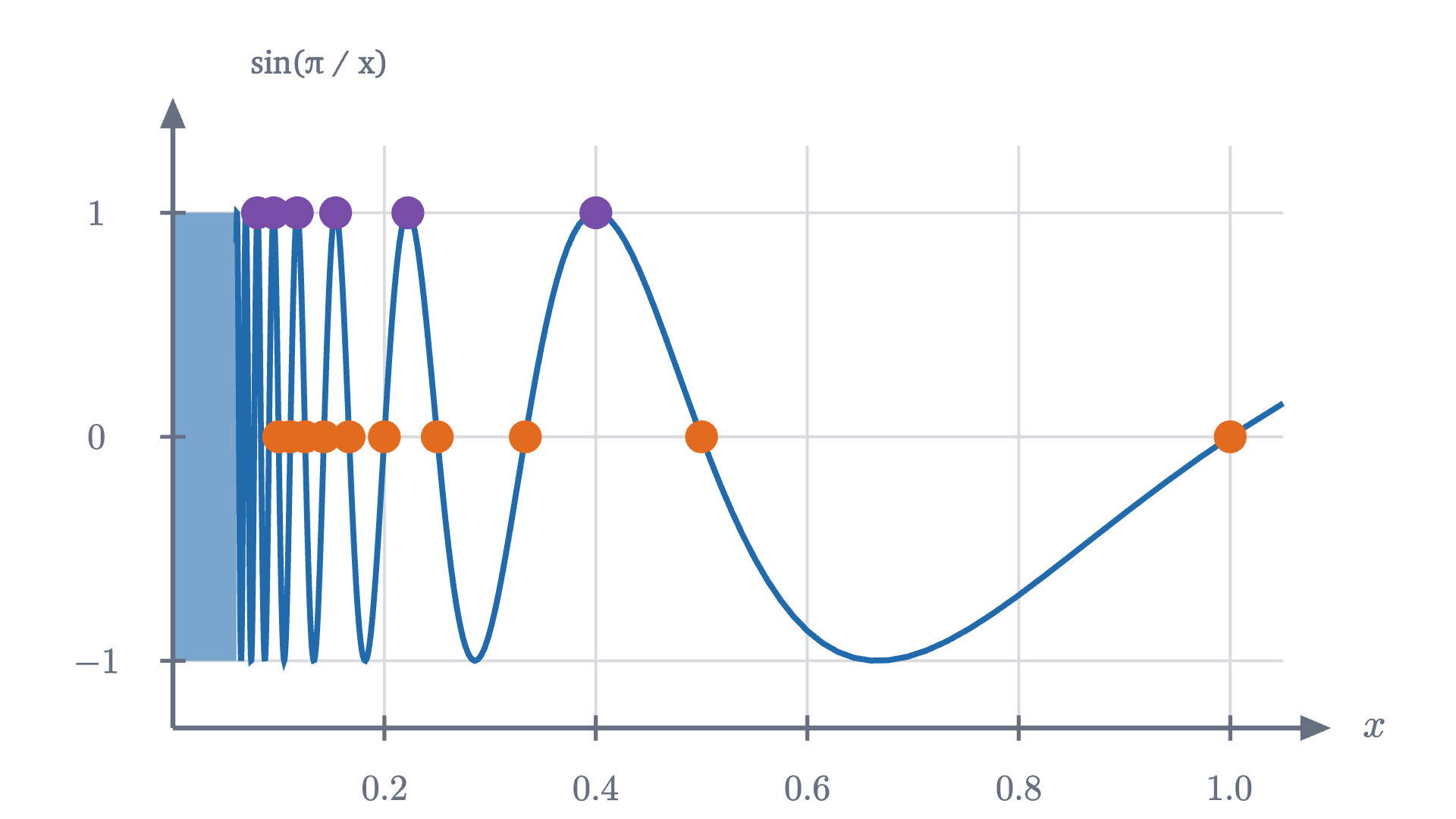
The graph of w(x) = \sin(\pi / x) for 0 < x \le 1. The orange dots are inputs where w is 0 and the purple dots are inputs where it is 1; both kinds crowd toward x = 0. Left of x = 0.06 the waves are too narrow to draw and are shown as a solid block.
The graph of $w(x) = \sin(\pi / x)$ for $0 < x \le 1$. The orange dots are inputs where $w$ is 0 and the purple dots are inputs where it is 1; both kinds crowd toward $x = 0$. Left of $x = 0.06$ the waves are too narrow to draw and are shown as a solid block.
Monocurl source
let fw = Wide(0, 1.05, -1.3, 1.3)
let LO = 0.06
mesh grid = GridLines(fw, [0.2, 0.4, 0.6, 0.8, 1], [-1, 0, 1])
mesh core = Region([at(fw, 0, -1), at(fw, LO, -1), at(fw, LO, 1), at(fw, 0, 1)], tint(AZURE, 0.6))
mesh curve = stroke{AZURE, 3} Polyline(map(sample(1 / 1.05, 1 / LO, 420), |t| at(fw, 1 / t, sin(PI * t))))
mesh axes = EdgeAxes(fw, [0.2, 0.4, 0.6, 0.8, 1], [-1, 0, 1], "x", "sin(π / x)", 1, 0, 0.8)
mesh zeros = map([1, 0.5, 1 / 3, 0.25, 0.2, 1 / 6, 1 / 7, 0.125, 1 / 9, 0.1], |x| Pt(at(fw, x, 0), EMBER, 0.085))
mesh tops = map([0.4, 2 / 9, 2 / 13, 2 / 17, 2 / 21, 0.08], |x| Pt(at(fw, x, 1), PLUM, 0.085))

Uses the shared definitions for this lesson's figures.

The graph explains the contradiction. As $x$ shrinks toward 0, $\frac{\pi}{x}$ grows without bound, so the sine runs through its cycle over and over, faster each time. Between any small positive number and 0 the function takes the value 0 infinitely often and the value 1 infinitely often. A table samples a few inputs, and by choosing them we chose the answer.

So “the values at the inputs I tried seem to settle” cannot be what a limit means. Whatever the definition is, it must speak about all inputs near the point, and it has to distinguish $\frac{\sin x}{x}$, which behaves, from $\sin\frac{\pi}{x}$, which does not.

A game: you name a tolerance, I name a window

To find the right statement, go back to a case where we understand everything. In lesson 1 a dropped ball had fallen $s(t) = 5t^2$ meters after $t$ seconds. Its average speed between time 1 and a different time $x$ is distance over time,

$$ f(x) = \frac{s(x) - s(1)}{x - 1} = \frac{5x^2 - 5}{x - 1} = \frac{5(x-1)(x+1)}{x - 1} = 5x + 5 \qquad (x \neq 1), $$

in meters per second. At $x = 1$ the quotient is $\frac{0}{0}$ and $f$ has no value. Everywhere else its graph is the line $5x + 5$, so its values near $x = 1$ are near 10.

Now suppose you doubt that 10 deserves to be called the limit, and you test me. You name a tolerance, say 1 m/s, and demand that the average speed be within that tolerance of 10. My job is to answer with a window around $x = 1$ such that every input in the window, other than 1 itself, meets your demand.

Since $f(x) - 10 = 5x - 5 = 5(x - 1)$, the distance from $f(x)$ to 10 is exactly five times the distance from $x$ to 1. To keep the first below 1, I need the second below $0.2$. So I answer “within $0.2$ of 1”, and I win that round.

  1. You demand an average speed within 1 m/s of 10. That is the green band from 9 to 11.
  2. I answer with a window: every x within 0.2 of 1 has its point on the graph inside the band.
  3. You tighten the tolerance to 0.5. I shrink the window to 0.1.
  4. You tighten to 0.25. I answer 0.05. One fifth of your tolerance always works.
The average speed $f(x) = 5x + 5$ for $x \ne 1$. Each time the tolerance band around 10 is tightened, a narrower window around $x = 1$ keeps the graph inside the band.
Monocurl source
let fg = Side(0.6, 1.4, 8, 12)
let Game = |eps, del| {
    var reply = []
    if (del > 0.001) {
        reply = [
            center{[3.0, -0.48, 0]} Cap("my window", 0.74, EMBER),
            center{[3.0, -0.98, 0]} scale{1.35} color{EMBER} Number(del, 2)
        ]
    }
    return [
        Band(fg, 10, eps),
        Window(fg, 1, del),
        center{[3.0, 0.72, 0]} scale{1.35} color{LEAF} Number(eps, 2),
        reply
    ]
}
mesh grid = GridLines(fg, [0.8, 1, 1.2], [9, 10, 11])
mesh game = Game(eps: 1, del: 0)
mesh axes = EdgeAxes(fg, [0.8, 1, 1.2], [9, 10, 11], "x", "average speed (m/s)", 1, 0, 1.45)
mesh curve = Graph(fg, |x| 5 * x + 5, 0.62, 1.38)
mesh hole = Ring(at(fg, 1, 10), AZURE, 0.11, 3.5)
mesh labels = center{[3.0, 1.22, 0]} Cap("your tolerance", 0.74, LEAF)

slide "You demand an average speed within 1 m/s of 10. That is the green band from 9 to 11."
    play Fade(0.6)

slide "I answer with a window: every x within 0.2 of 1 has its point on the graph inside the band."
    game.del = 0.2
    play Lerp(1.2, [&game])

slide "You tighten the tolerance to 0.5. I shrink the window to 0.1."
    game.eps = 0.5
    play Lerp(1, [&game])
    game.del = 0.1
    play Lerp(1, [&game])

slide "You tighten to 0.25. I answer 0.05. One fifth of your tolerance always works."
    game.eps = 0.25
    play Lerp(1, [&game])
    game.del = 0.05
    play Lerp(1, [&game])

Uses the shared definitions for this lesson's figures.

Pause and try

You tighten the tolerance to $0.001$ m/s. What window do I answer with? Then give my reply to a general tolerance, written as a letter.

Show answerHide answer

I need $5|x - 1| < 0.001$, so $|x - 1| < 0.0002$: any end time within two ten-thousandths of a second of 1. For a general tolerance $\varepsilon > 0$, the window “within $\varepsilon / 5$ of 1” works, because then $|f(x) - 10| = 5|x - 1| < 5 \cdot \frac{\varepsilon}{5} = \varepsilon$.

I have a winning reply to every tolerance you could name, and that is the content of “the limit is 10”. A limit is a guarantee: closeness of the output, to any standard, can be bought by closeness of the input.

The definition

Written with the traditional letters, $\varepsilon$ (epsilon) for the tolerance and $\delta$ (delta) for the half-width of the window, the game becomes the definition.

Each clause is a rule of the game. “For every $\varepsilon > 0$” says you may name any tolerance. “There is a $\delta > 0$” says I must be able to reply, with a $\delta$ that may depend on your $\varepsilon$. The inequality $|x - a| < \delta$ describes the window, on both sides of $a$. The inequality $0 < |x - a|$ removes $x = a$ from the window, so the definition never looks at $f(a)$: the function may be undefined there, as ours are, or may have some unrelated value. And “implies” says that every input in the window must succeed, which is the clause that a table of values cannot check.

This is the definition from lesson 1 with new letters: there the variable was $h$ and the point was 0. We also showed there that a function cannot have two different limits at one point, so “the limit” is a single number when it exists. I will write $f(x) \to L$ as $x \to a$ for the same statement.

For the average speed, the reply $\delta = \varepsilon / 5$ proves $\lim_{x \to 1} f(x) = 10$. That function was a straight line, so the output error was a fixed multiple of the input error. On a curve it is not, and the reply takes one more idea.
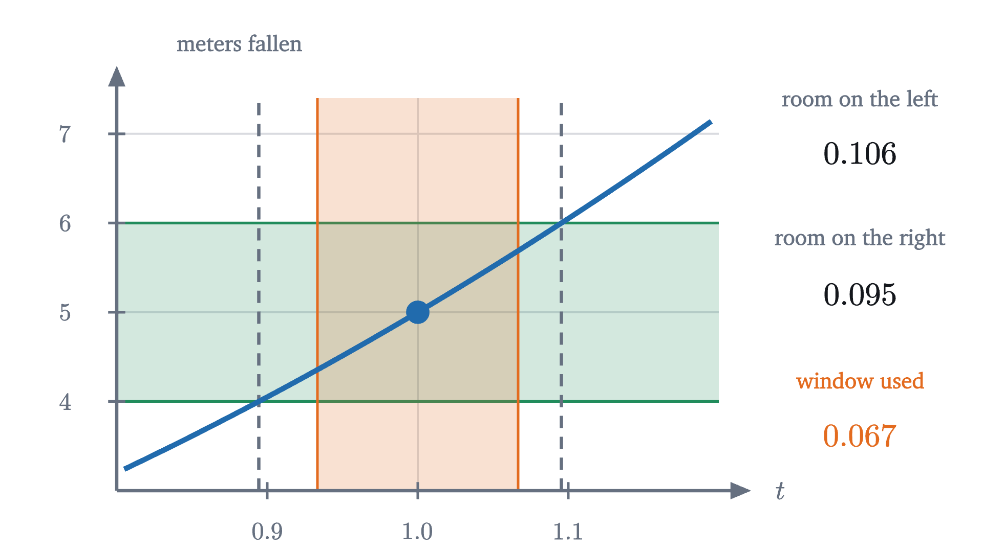
The distance 5t^2 near t = 1 with the tolerance band from 4 to 6 meters. The curve stays in the band between the dashed lines, which are not the same distance from t = 1. The orange window of half-width 1/15 from the proof sits safely inside them.
The distance $5t^2$ near $t = 1$ with the tolerance band from 4 to 6 meters. The curve stays in the band between the dashed lines, which are not the same distance from $t = 1$. The orange window of half-width $1/15$ from the proof sits safely inside them.
Monocurl source
let fc = Side(0.8, 1.2, 3, 7.4)
let s = |t| 5 * t * t
let TL = sqrt(0.8)
let TR = sqrt(1.2)
mesh grid = GridLines(fc, [1], [4, 5, 6, 7])
mesh band = Band(fc, 5, 1)
mesh window = Window(fc, 1, 1 / 15)
mesh edges = [
    stroke{SLATE, 2.5} dashed{[0.1, 0.07]} Line(at(fc, TL, 3), at(fc, TL, 7.4)),
    stroke{SLATE, 2.5} dashed{[0.1, 0.07]} Line(at(fc, TR, 3), at(fc, TR, 7.4))
]
mesh axes = EdgeAxes(fc, [0.9, 1, 1.1], [4, 5, 6, 7], "t", "meters fallen", 1, 0, 1.0)
mesh curve = Graph(fc, s, 0.805, 1.195)
mesh dot = Pt(at(fc, 1, 5), AZURE, 0.09)
mesh labels = [
    center{[3.0, 1.45, 0]} Note("room on the left", 0.72),
    center{[3.0, 1.0, 0]} Math(to_string(1 - TL, 3), 0.95),
    center{[3.0, 0.3, 0]} Note("room on the right", 0.72),
    center{[3.0, -0.15, 0]} Math(to_string(TR - 1, 3), 0.95),
    center{[3.0, -0.85, 0]} Cap("window used", 0.72, EMBER),
    center{[3.0, -1.3, 0]} Math(to_string(1 / 15, 3), 0.95, EMBER)
]

Uses the shared definitions for this lesson's figures.

The window from the proof is not the largest that works: the curve stays in the band out to $0.106$ on the left and $0.095$ on the right, and we used $0.067$. That is fine. The definition asks for a $\delta$, and any smaller one also works, so there is no need to find the best. The device of taking “the smaller of two numbers” makes two promises at once: a rough one ($|t - 1| < 1$) that tames the nuisance factor, and a fine one that then wins the round. Every proof below uses it.

When there is no limit

To prove that a limit does not exist we need the opposite of the definition, stated just as carefully.

Pause and try

The definition says “for every $\varepsilon > 0$ there is a $\delta > 0$ such that every $x$ with $0 < |x - a| < \delta$ has $|f(x) - L| < \varepsilon$.” Write down what it means for this to be false. Who has to produce what?

Show answerHide answer

It is false when you have a winning tolerance: there is an $\varepsilon > 0$ such that for every $\delta > 0$, some $x$ with $0 < |x - a| < \delta$ has $|f(x) - L| \ge \varepsilon$. You produce one tolerance, and for whatever window I offer you point to one input inside it that misses. To show there is no limit at all, do this for every candidate $L$.

The simplest function with no limit has a jump. Let $u(x) = 0$ for $x < 0$ and $u(x) = 1$ for $x > 0$.

  1. Candidate L = 1. Inputs to the right of 0 land in the band. Inputs to the left give 0, which misses, and a narrower window would not help.
  2. Candidate L = 0. Now the left side is fine and every input on the right misses.
  3. Candidate L = 0.5. Both sides miss. A band of height 0.8 cannot contain two values that are 1 apart.
A function that jumps from 0 to 1 at $x = 0$, with a tolerance of 0.4 and a window of half-width 0.3. For each candidate limit $L$, the red part of the graph is inside the window and outside the band.
Monocurl source
let fj = Side(-1, 1, -0.6, 1.6)
let Try = |L| {
    var lc = ROSE
    var rc = ROSE
    if (abs(L) < 0.4) {
        lc = LEAF
    }
    if (abs(1 - L) < 0.4) {
        rc = LEAF
    }
    return [
        Band(fj, L, 0.4),
        Window(fj, 0, 0.3),
        Seg(at(fj, -1, 0), at(fj, 0, 0), AZURE, 4),
        Seg(at(fj, 0, 1), at(fj, 1, 1), AZURE, 4),
        Seg(at(fj, -0.3, 0), at(fj, 0, 0), lc, 7),
        Seg(at(fj, 0, 1), at(fj, 0.3, 1), rc, 7),
        Ring(at(fj, 0, 0), AZURE, 0.1, 3.5),
        Ring(at(fj, 0, 1), AZURE, 0.1, 3.5),
        center{[3.0, 0.55, 0]} scale{1.35} color{LEAF} Number(L, 2)
    ]
}
mesh grid = GridLines(fj, [-0.5, 0, 0.5], [0, 0.5, 1])
mesh attempt = Try(L: 1)
mesh axes = EdgeAxes(fj, [-0.5, 0, 0.5], [0, 0.5, 1], "x", "u(x)", 1, 1, 0.5)
mesh labels = [
    center{[3.0, 1.05, 0]} Cap("candidate L", 0.74, LEAF),
    center{[3.0, -0.4, 0]} Note("tolerance 0.4", 0.74),
    center{[3.0, -0.85, 0]} Note("window 0.3", 0.74)
]

slide "Candidate L = 1. Inputs to the right of 0 land in the band. Inputs to the left give 0, which misses, and a narrower window would not help."
    play Fade(0.6)

slide "Candidate L = 0. Now the left side is fine and every input on the right misses."
    attempt.L = 0
    play Lerp(1.6, [&attempt])

slide "Candidate L = 0.5. Both sides miss. A band of height 0.8 cannot contain two values that are 1 apart."
    attempt.L = 0.5
    play Lerp(1.6, [&attempt])

Uses the shared definitions for this lesson's figures.

The last slide is the proof. If $u$ had a limit $L$ at 0, then for $\varepsilon = 0.4$ some window would put every $u(x)$ within $0.4$ of $L$. Every window contains negative inputs, where $u = 0$, and positive inputs, where $u = 1$, so $L$ would be within $0.4$ of both 0 and 1, which no number is.

What $u$ does have is a limit from each side. Testing only inputs with $a < x < a + \delta$ gives the right-hand limit $\lim_{x \to a^+} f(x)$, and only inputs with $a - \delta < x < a$ the left-hand limit $\lim_{x \to a^-} f(x)$. For $u$ at 0 these are 1 and 0. A two-sided limit exists exactly when both one-sided limits exist and are equal: a window that works on both sides works on each, and given a $\delta$ for each side, the smaller of the two works on both.

A jump is a mild failure. The function $w(x) = \sin\frac{\pi}{x}$ fails more thoroughly: it has no limit at 0 even from one side. Watch what zooming in does to its graph.

Zooming in on $w(x) = \sin(\pi / x)$ at $x = 0$. However narrow the window becomes, the graph inside it still reaches both 1 and $-1$, so it never fits inside the green band of tolerance 0.5.
Monocurl source
mesh view = Zoom(w: 1, 0)
mesh axes = ZoomAxes("sin(π / x)")

slide "zoom"
    play Wait(0.8)
    view.w = 0.25
    play Lerp(6, [&view], |u| (1 - 0.25 ^ u) / 0.75)
    play Wait(1.5)

Uses the shared definitions for this lesson's figures.

To turn that picture into a proof we need one tool, which every later argument uses as well.

Its usual job is to pass through an intermediate point: the distance from $A$ to $C$ is at most the distance from $A$ to $B$ plus the distance from $B$ to $C$, that is, $|A - C| \le |A - B| + |B - C|$ (take $p = A - B$ and $q = B - C$).

The limit laws

Finding a $\delta$ by hand for every new function would be slow. In practice limits are computed from a few known ones by rules, the ones that lessons 1 to 4 quoted. Before stating them, try the numbers.

Pause and try

A quantity $f$ is known to be within $0.01$ of 3, and a quantity $g$ is within $0.01$ of 4. How far can $f + g$ be from 7? How far can $f \cdot g$ be from 12?

Show answerHide answer

The sum lies between $2.99 + 3.99 = 6.98$ and $3.01 + 4.01 = 7.02$, so it is within $0.02$ of 7: the errors add. The product lies between $2.99 \times 3.99 = 11.9301$ and $3.01 \times 4.01 = 12.0701$, so it is within $0.0701$ of 12. That is about $0.01 \times 4 + 0.01 \times 3$: each error is multiplied by the size of the other quantity.

For the sum, the errors add, so to hold the sum within $\varepsilon$ it is enough to hold each term within $\varepsilon / 2$. The product needs a picture. Draw the target as a rectangle of height $L$ and width $M$, and the actual product as a rectangle of height $f$ and width $g$.

  1. The target is a rectangle of height L = 3 and width M = 4, with area 12.
  2. The actual f and g are a little off: 3.3 and 4.5. The product is 14.85, too big by 2.85.
  3. The excess is two strips. Across the top: (f - L) times g. Down the side: L times (g - M).
  4. Shrink both errors and both strips shrink with them, as long as the width g of the top strip stays bounded.
A product $f \cdot g$ compared with its target $L \cdot M = 3 \times 4$, with the errors exaggerated. The excess area is a strip across the top of area $(f - L)\,g$ and a strip down the side of area $L\,(g - M)$.
Monocurl source
let RO = [-3.6, -2.0, 0]
let RS = 1.08
let Cell = |x0, y0, x1, y1, col, amount| Shape([
    [RO[0] + RS * x0, RO[1] + RS * y0, 0],
    [RO[0] + RS * x1, RO[1] + RS * y0, 0],
    [RO[0] + RS * x1, RO[1] + RS * y1, 0],
    [RO[0] + RS * x0, RO[1] + RS * y1, 0]
], col, amount, 3)
let Rects = |ef, eg| {
    var parts = [Cell(0, 0, 4, 3, SLATE, 0.14)]
    if (ef > 0.005) {
        parts .= Cell(0, 3, 4 + eg, 3 + ef, AZURE, 0.4)
        parts .= Cell(4, 0, 4 + eg, 3, EMBER, 0.4)
    }
    return [
        parts,
        center{[3.35, 1.45, 0]} scale{1.25} color{AZURE} Number(3 + ef, 2),
        center{[3.35, 0.85, 0]} scale{1.25} color{EMBER} Number(4 + eg, 2),
        center{[3.0, -1.5, 0]} scale{1.35} color{INK} Number((3 + ef) * (4 + eg) - 12, 2)
    ]
}
mesh rects = Rects(ef: 0, eg: 0)
mesh fixed = [
    center{[RO[0] + RS * 2, RO[1] + RS * 1.5, 0]} Math("L \cdot M = 12", 1.0, SLATE),
    center{[2.65, 1.45, 0]} Math("f =", 0.9, AZURE),
    center{[2.65, 0.85, 0]} Math("g =", 0.9, EMBER),
    center{[3.0, -1.0, 0]} Math("fg - LM", 0.9)
]
mesh names = []

slide "The target is a rectangle of height L = 3 and width M = 4, with area 12."
    play Fade(0.6)

slide "The actual f and g are a little off: 3.3 and 4.5. The product is 14.85, too big by 2.85."
    rects.ef = 0.3
    rects.eg = 0.5
    play Lerp(1.4, [&rects])

slide "The excess is two strips. Across the top: (f - L) times g. Down the side: L times (g - M)."
    names = [
        center{[RO[0] + RS * 2.25, RO[1] + RS * 3.3 + 0.36, 0]} Math("(f - L) \cdot g", 0.9, AZURE),
        center{[RO[0] + RS * 4.5 + 0.75, RO[1] + RS * 1.5, 0]} Math("L \cdot (g - M)", 0.85, EMBER)
    ]
    play Fade(0.5, [&names])

slide "Shrink both errors and both strips shrink with them, as long as the width g of the top strip stays bounded."
    rects.ef = 0.1
    rects.eg = 0.15
    play Lerp(1.8, [&rects])

Uses the shared definitions for this lesson's figures.

The picture gives an identity that is true for all numbers, whatever their signs:

$$ fg - LM = (f - L)\,g + L\,(g - M). $$

The second strip is easy: $L$ is a constant, so $L(g - M)$ is small when $g - M$ is. The first strip is a small quantity $f - L$ multiplied by $g$, which is not a constant. This is the nuisance factor from the $5t^2$ example again, and the same repair works: near $a$, the function $g$ is within 1 of $M$, so its size is less than $|M| + 1$.

Two limits are needed to get started, and both are immediate: a constant function $c$ has limit $c$, and $\lim_{x \to a} x = a$ (reply $\delta = \varepsilon$). Every polynomial is built from constants and $x$ by sums and products, so the laws give $\lim_{x \to a} p(x) = p(a)$ for every polynomial $p$, and the quotient law extends this to ratios of polynomials wherever the denominator is not zero at $a$.

This settles a debt from lesson 1, where the difference quotient of $\frac{1}{x}$ was $\frac{-1}{a(a+h)}$ and its limit $-\frac{1}{a^2}$ was taken “by the quotient law”: the denominator is a polynomial in $h$ with limit $a^2 \neq 0$.

The squeeze theorem

The laws do not reach the function we started with. In $\frac{\sin x}{x}$ the denominator has limit 0, and there is no algebra that cancels an $x$ out of $\sin x$. What we do have, from the geometry in lesson 4, is a pair of bounds. Comparing the areas of a triangle, a circular sector and a larger triangle gave $\sin x < x < \tan x$ for $0 < x < \frac{\pi}{2}$, and from that
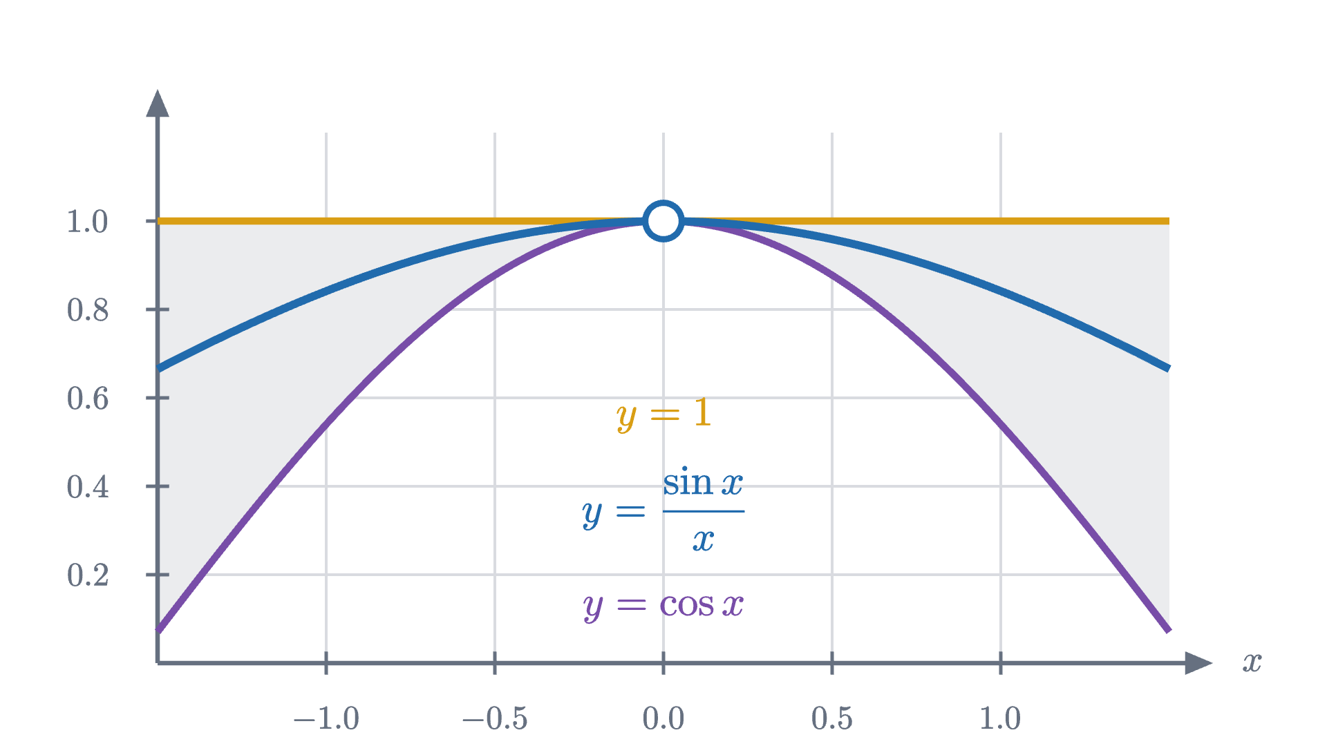
$$ \cos x < \frac{\sin x}{x} < 1 \qquad \text{for } 0 < |x| < \frac{\pi}{2}. $$
Near x = 0 the graph of \frac{\sin x}{x} (blue, with a hole at 0) runs between the graph of \cos x below it and the horizontal line at height 1 above it. Both of those reach height 1 at x = 0.
Near $x = 0$ the graph of $\frac{\sin x}{x}$ (blue, with a hole at 0) runs between the graph of $\cos x$ below it and the horizontal line at height 1 above it. Both of those reach height 1 at $x = 0$.
Monocurl source
let fq = Wide(-1.5, 1.5, 0, 1.2)
mesh grid = GridLines(fq, [-1, -0.5, 0, 0.5, 1], [0.2, 0.4, 0.6, 0.8, 1])
mesh corridor = block {
    var pts = [at(fq, -1.5, 1), at(fq, 1.5, 1)]
    for (x in sample(1.5, -1.5, 60)) {
        pts .= at(fq, x, cos(x))
    }
    . Region(pts, tint(SLATE, 0.13))
}
mesh axes = EdgeAxes(fq, [-1, -0.5, 0, 0.5, 1], [0.2, 0.4, 0.6, 0.8, 1], "x", "", 1, 1)
mesh bounds = [
    Seg(at(fq, -1.5, 1), at(fq, 1.5, 1), GOLD, 4),
    Graph(fq, cos, -1.5, 1.5, PLUM, 4)
]
mesh curve = Graph(fq, sinc, -1.5, 1.5, AZURE, 4.5)
mesh hole = Ring(at(fq, 0, 1), AZURE, 0.11, 3.5)
mesh legend = [
    center{at(fq, 0, 0.56)} Math("y = 1", 0.9, GOLD),
    center{at(fq, 0, 0.35)} Math("y = \frac{\sin x}{x}", 0.9, AZURE),
    center{at(fq, 0, 0.12)} Math("y = \cos x", 0.9, PLUM)
]

Uses the shared definitions for this lesson's figures.

The function is trapped in a corridor whose floor and ceiling both arrive at height 1. That argument does not depend on what the trapped function is.

The theorem does not assume that $f$ has a limit; that is its conclusion. To apply it to $\frac{\sin x}{x}$ we need the limits of the two bounds. The ceiling is the constant 1. For the floor, lesson 4 also proved $0 \le 1 - \cos x \le \frac{x^2}{2}$ for every $x$, that is,

$$ 1 - \frac{x^2}{2} \le \cos x \le 1. $$

Both outer functions are polynomials with limit 1 at 0, so by the squeeze theorem $\lim_{x \to 0} \cos x = 1$. A second application, to $\cos x < \frac{\sin x}{x} < 1$, gives

$$ \lim_{x \to 0} \frac{\sin x}{x} = 1. $$

The squeeze theorem and the limit laws are proved above; the two inequalities are quoted from lesson 4, where they were proved from the area of a circular sector.

The squeeze theorem can even tame the function that had no limit.

Zooming in on $x \sin(\pi / x)$ at $x = 0$ with the vertical scale held fixed. The graph still oscillates without end, but it is trapped between the lines $y = |x|$ and $y = -|x|$, which close down onto 0.
Monocurl source
mesh view = Zoom(w: 1, 1)
mesh axes = ZoomAxes("x sin(π / x)")

slide "zoom"
    play Wait(0.8)
    view.w = 0.25
    play Lerp(6, [&view], |u| (1 - 0.25 ^ u) / 0.75)
    play Wait(1.5)

Uses the shared definitions for this lesson's figures.

The function still oscillates infinitely often in every window around 0, so oscillation alone does not destroy a limit. What matters is whether the size of the oscillation inside the window can be forced below any tolerance.

Continuity

For a polynomial $p$ we found $\lim_{x \to a} p(x) = p(a)$: the limit is the value. That property has a name, and the next lessons depend on it.

The definition makes three demands: $f(a)$ exists, the limit exists, and they are equal. The jump function $u$ fails the second at 0. The function $\frac{\sin x}{x}$ fails only the first: define its value at 0 to be 1 and it becomes continuous there. By the limit laws, sums, products and quotients (with nonzero denominator) of continuous functions are continuous.

Check yourself

Let $f(x) = \dfrac{x^2 - 4}{x - 2}$ for $x \neq 2$, and let $f(2) = 0$. What is $\lim_{x \to 2} f(x)$?

What was hard

The difficulty is the order of the words: “for every tolerance there is a window” is a promise that can be kept or broken. With the definition fixed, the proofs share one pattern: split the error with the triangle inequality, give each piece a share of $\varepsilon$, and take the smallest window. The integral, defined in the next lesson, is a limit of the same kind.

Problems

The first two repeat the lesson’s moves, the next three ask you to combine them or to explain, and the last goes further.

Problem 1

Prove from the definition that $\lim_{x \to 2} (5x - 3) = 7$. What window does your proof give for the tolerance $\varepsilon = 0.01$?

Show solutionHide solution

$|(5x - 3) - 7| = |5x - 10| = 5|x - 2|$. Given $\varepsilon > 0$, let $\delta = \varepsilon / 5$. If $0 < |x - 2| < \delta$ then $|(5x - 3) - 7| = 5|x - 2| < 5\delta = \varepsilon$. For $\varepsilon = 0.01$ this is $\delta = 0.002$. At the edge, $x = 2.002$ gives $5x - 3 = 7.01$, exactly at the tolerance, so inputs strictly inside the window are strictly within it.

Problem 2

Use the limit laws to evaluate (a) $\displaystyle\lim_{x \to 2} \frac{x^2 + 3x}{x - 1}$ and (b) $\displaystyle\lim_{x \to 1} \frac{x^2 + 3x - 4}{x - 1}$. Say which law is used at each step, and why (b) needs an extra step.

Show solutionHide solution

(a) The numerator is a polynomial, so by the sum and product laws its limit at 2 is $4 + 6 = 10$. The denominator has limit $2 - 1 = 1 \neq 0$. By the quotient law the limit is $\frac{10}{1} = 10$. (b) The denominator has limit 0, so the quotient law does not apply. Factor: $x^2 + 3x - 4 = (x - 1)(x + 4)$, so the quotient equals $x + 4$ for every $x \neq 1$. Functions that agree for $x \neq 1$ have the same limit at 1, and $x + 4$ has limit 5. Check at $x = 1.1$: $\frac{0.51}{0.1} = 5.1$.

Problem 3

Prove directly from the definition, without the quotient law, that $\lim_{x \to 2} \dfrac{1}{x} = \dfrac{1}{2}$.

Show solutionHide solution

$\left|\frac{1}{x} - \frac{1}{2}\right| = \frac{|2 - x|}{2|x|}$. The nuisance factor is $\frac{1}{|x|}$, which is large if $x$ is near 0. Promise $|x - 2| < 1$; then $x > 1$, so $\frac{1}{|x|} < 1$ and the error is less than $\frac{|x - 2|}{2}$. Given $\varepsilon > 0$, let $\delta$ be the smaller of $1$ and $2\varepsilon$. If $0 < |x - 2| < \delta$ then $\left|\frac{1}{x} - \frac{1}{2}\right| < \frac{|x - 2|}{2} < \frac{2\varepsilon}{2} = \varepsilon$. The promise $|x - 2| < 1$ plays the part of $|g(x) - M| < \frac{|M|}{2}$ in the proof of the quotient law: it keeps the denominator away from 0.

Problem 4

Show that $\dfrac{1}{x}$ has no limit as $x \to 0$. (This is a third way to fail, different from a jump and from oscillation.)

Show solutionHide solution

Suppose the limit were $L$. Take $\varepsilon = 1$; there would be a $\delta > 0$ such that $0 < |x| < \delta$ implies $\left|\frac{1}{x} - L\right| < 1$. Choose a positive $x$ smaller than both $\delta$ and $\frac{1}{|L| + 1}$. Then $\frac{1}{x} > |L| + 1$. By the triangle inequality $\frac{1}{x} = \left|\frac{1}{x}\right| \le \left|\frac{1}{x} - L\right| + |L|$, so $\left|\frac{1}{x} - L\right| \ge \frac{1}{x} - |L| > 1$. That input is in the window and misses the tolerance, a contradiction. The function fails by growing without bound.

Problem 5

Here is a “proof” that $1 = 0$. Find the error. “For $x \neq 0$ we have $x \cdot \frac{1}{x} = 1$, so $\lim_{x \to 0} x \cdot \frac{1}{x} = 1$. By the product law, $\lim_{x \to 0} x \cdot \frac{1}{x} = \left(\lim_{x \to 0} x\right)\left(\lim_{x \to 0} \frac{1}{x}\right) = 0 \cdot \left(\lim_{x \to 0} \frac{1}{x}\right) = 0$.”

Show solutionHide solution

The product law has a hypothesis: both limits must exist. By the previous problem $\lim_{x \to 0} \frac{1}{x}$ does not exist, so the law says nothing here and the second chain of equalities has no meaning from its second step on. “Zero times anything is zero” applies to numbers, and $\lim_{x \to 0} \frac{1}{x}$ is not a number. In the proof of the product law, the hypothesis was used when we bounded $|g(x)|$ by $|M| + 1$ near $a$; the function $\frac{1}{x}$ has no such bound near 0.

Problem 6

Let $f(x) = x^2 \sin\dfrac{\pi}{x}$ for $x \neq 0$ and $f(0) = 0$. (a) Show that $f$ is continuous at 0. (b) Show that $f$ is differentiable at 0 and find $f'(0)$.

Show solutionHide solution

(a) For $x \neq 0$, $\left|\sin\frac{\pi}{x}\right| \le 1$ gives $-x^2 \le f(x) \le x^2$. Both $x^2$ and $-x^2$ are polynomials with limit 0 at 0, so by the squeeze theorem $\lim_{x \to 0} f(x) = 0 = f(0)$. (b) The difference quotient at 0 is $\frac{f(h) - f(0)}{h} = \frac{h^2 \sin(\pi / h)}{h} = h \sin\frac{\pi}{h}$ for $h \neq 0$. By the worked example in the lesson this has limit 0 as $h \to 0$. So $f'(0) = 0$. The graph oscillates infinitely often near 0 and still has a tangent line there, the $x$ axis, because it is trapped between $\pm x^2$.

Shared definitions used by this lesson's figures
# house kit: prepended to every essay figure after the std imports

# palette. AZURE and EMBER are the two actors, LEAF marks an answer, ROSE a problem
let PAPER = [1, 1, 1, 1]
let INK = [0.08, 0.09, 0.11, 1]
let SLATE = [0.40, 0.44, 0.50, 1]
let MIST = [0.85, 0.86, 0.88, 1]
let AZURE = [0.13, 0.42, 0.68, 1]
let EMBER = [0.89, 0.42, 0.12, 1]
let LEAF = [0.13, 0.55, 0.36, 1]
let ROSE = [0.78, 0.22, 0.24, 1]
let PLUM = [0.47, 0.30, 0.66, 1]
let GOLD = [0.85, 0.62, 0.08, 1]

background = PAPER

# an opaque pastel of col; use for fills so overlaps do not darken
let tint = |col, amount = 0.18| [
    1 - (1 - col[0]) * amount,
    1 - (1 - col[1]) * amount,
    1 - (1 - col[2]) * amount,
    1
]

# text: Cap for labels, Note for quiet labels, Math for typeset maths
let Cap = |txt, size = 0.75, col = INK| color{col} Text(txt, size, "Charter")
let Note = |txt, size = 0.65| color{SLATE} Text(txt, size, "Charter")
let Math = |tex, size = 0.9, col = INK| color{col} Tex(tex, size)

# a paper rectangle to sit behind text that crosses lines
let Plate = |pos, size| center{pos} fill{PAPER} stroke{alpha{0} PAPER, 0} Rect(size)

# shapes with fill and stroke both set, so no stray black appears
let Pt = |pos, col = INK, r = 0.075| center{pos} fill{col} stroke{col, 1} Circle(r, 48)
let Ring = |pos, col = INK, r = 0.1, w = 3| center{pos} fill{PAPER} stroke{col, w} Circle(r, 48)
let Seg = |a, b, col = INK, w = 3| stroke{col, w} Line(a, b)
let Path = |pts, col = INK, w = 3| stroke{col, w} Polyline(pts)
let Region = |pts, col| fill{col} stroke{alpha{0} col, 0} Polygon(pts)
let Outline = |pts, col = INK, w = 3| fill{alpha{0} PAPER} stroke{col, w} Polygon(pts)
let Shape = |pts, col, amount = 0.18, w = 3| fill{tint(col, amount)} stroke{col, w} Polygon(pts)
let Disc = |pos, r, col, amount = 0.18, w = 3| center{pos} fill{tint(col, amount)} stroke{col, w} Circle(r, 96)
let Box = |pos, size, col, amount = 0.18, w = 3| center{pos} fill{tint(col, amount)} stroke{col, w} Rect(size)
# a line from a to b ending in a small solid arrowhead
let Tip = |a, b, col = INK, w = 3, head = 0.17| {
    let d = normalize([b[0] - a[0], b[1] - a[1], 0])
    let n = [-d[1], d[0], 0]
    let base = [b[0] - d[0] * head, b[1] - d[1] * head, 0]
    return [
        stroke{col, w} Line(a, base),
        fill{col} stroke{col, 1} Polygon([
            b,
            [base[0] + n[0] * head * 0.42, base[1] + n[1] * head * 0.42, 0],
            [base[0] - n[0] * head * 0.42, base[1] - n[1] * head * 0.42, 0]
        ])
    ]
}

# plots. a frame is [x0, x1, y0, y1, centre, width, height]: a data window and the scene box it fills
let Frame = |x0, x1, y0, y1, c = [0, 0, 0], w = 6.4, h = 3.6| [x0, x1, y0, y1, c, w, h]
let fx = |fr, x| fr[4][0] + (x - (fr[0] + fr[1]) / 2) * fr[5] / (fr[1] - fr[0])
let fy = |fr, y| fr[4][1] + (y - (fr[2] + fr[3]) / 2) * fr[6] / (fr[3] - fr[2])
let at = |fr, x, y| [fx(fr, x), fy(fr, y), 0]

# axes through the data origin (or the nearest edge of the window), with optional names
let Axes = |fr, x_name = "", y_name = "", col = SLATE| {
    let ox = clamp(fr[0], 0, fr[1])
    let oy = clamp(fr[2], 0, fr[3])
    var parts = [
        Tip(at(fr, fr[0], oy), [fx(fr, fr[1]) + 0.25, fy(fr, oy), 0], col, 2.5, 0.15),
        Tip(at(fr, ox, fr[2]), [fx(fr, ox), fy(fr, fr[3]) + 0.25, 0], col, 2.5, 0.15)
    ]
    if (x_name != "") {
        parts .= center{[fx(fr, fr[1]) + 0.5, fy(fr, oy), 0]} Math(x_name, 0.8, col)
    }
    if (y_name != "") {
        parts .= center{[fx(fr, ox), fy(fr, fr[3]) + 0.5, 0]} Math(y_name, 0.8, col)
    }
    return parts
}

# tick marks with numbers at the listed data values
let XTicks = |fr, xs, col = SLATE, places = 0| block {
    let oy = fy(fr, clamp(fr[2], 0, fr[3]))
    for (x in xs) {
        . Seg([fx(fr, x), oy - 0.07, 0], [fx(fr, x), oy + 0.07, 0], col, 2)
        . center{[fx(fr, x), oy - 0.33, 0]} Math(to_string(x, places), 0.72, col)
    }
}
let YTicks = |fr, ys, col = SLATE, places = 0| block {
    let ox = fx(fr, clamp(fr[0], 0, fr[1]))
    for (y in ys) {
        . Seg([ox - 0.07, fy(fr, y), 0], [ox + 0.07, fy(fr, y), 0], col, 2)
        . center{[ox - 0.36, fy(fr, y), 0]} Math(to_string(y, places), 0.72, col)
    }
}

# faint grid lines at the listed data values
let GridLines = |fr, xs, ys, col = MIST| block {
    for (x in xs) {
        . Seg(at(fr, x, fr[2]), at(fr, x, fr[3]), col, 1.5)
    }
    for (y in ys) {
        . Seg(at(fr, fr[0], y), at(fr, fr[1], y), col, 1.5)
    }
}

# the graph of f over [a, b], drawn in the frame. values are clamped to the window
let Graph = |fr, f, a, b, col = AZURE, w = 4, n = 160|
    stroke{col, w} Polyline(map(sample(a, b, n), |x| at(fr, x, clamp(fr[2], f(x), fr[3]))))

# the region between the graph of f and the x axis over [a, b]
let AreaUnder = |fr, f, a, b, col = AZURE, amount = 0.2, n = 80| {
    var pts = [at(fr, a, 0)]
    for (x in sample(a, b, n)) {
        pts .= at(fr, x, clamp(fr[2], f(x), fr[3]))
    }
    pts .= at(fr, b, 0)
    return fill{tint(col, amount)} stroke{alpha{0} col, 0} Polygon(pts)
}

# sin(x)/x, with the gap at 0 filled in so that plotting never divides by zero
let sinc = |x| {
    if (abs(x) < 0.000001) {
        return 1
    }
    return sin(x) / x
}
# two layouts: a plot with a readout panel on its right, and a plot across the whole frame
let Side = |x0, x1, y0, y1| Frame(x0, x1, y0, y1, [-0.6, -0.15, 0], 4.9, 3.2)
let Wide = |x0, x1, y0, y1| Frame(x0, x1, y0, y1, [0, -0.15, 0], 6.1, 3.2)
# axes along the bottom and left edges of a frame, with numbered ticks and names
let EdgeAxes = |fr, xs, ys, x_name, y_name, xp = 0, yp = 0, y_dx = 0.9| block {
    let bx = fx(fr, fr[0])
    let by = fy(fr, fr[2])
    . Tip([bx, by, 0], [fx(fr, fr[1]) + 0.25, by, 0], SLATE, 2.5, 0.15)
    . Tip([bx, by, 0], [bx, fy(fr, fr[3]) + 0.25, 0], SLATE, 2.5, 0.15)
    for (x in xs) {
        . Seg([fx(fr, x), by - 0.07, 0], [fx(fr, x), by + 0.07, 0], SLATE, 2)
        . center{[fx(fr, x), by - 0.33, 0]} Math(to_string(x, xp), 0.72, SLATE)
    }
    for (y in ys) {
        . Seg([bx - 0.07, fy(fr, y), 0], [bx + 0.07, fy(fr, y), 0], SLATE, 2)
        . center{[bx - 0.42, fy(fr, y), 0]} Math(to_string(y, yp), 0.72, SLATE)
    }
    if (x_name != "") {
        . center{[fx(fr, fr[1]) + 0.5, by, 0]} Math(x_name, 0.8, SLATE)
    }
    if (y_name != "") {
        . center{[bx + y_dx, fy(fr, fr[3]) + 0.45, 0]} Note(y_name, 0.72)
    }
}
# the tolerance: a horizontal band of half-height eps about the level L
let Band = |fr, L, eps, col = LEAF| {
    let lo = max(fr[2], L - eps)
    let hi = min(fr[3], L + eps)
    return [
        fill{alpha{0.2} col} stroke{alpha{0} col, 0} Polygon([at(fr, fr[0], lo), at(fr, fr[1], lo), at(fr, fr[1], hi), at(fr, fr[0], hi)]),
        Seg(at(fr, fr[0], lo), at(fr, fr[1], lo), col, 2),
        Seg(at(fr, fr[0], hi), at(fr, fr[1], hi), col, 2)
    ]
}
# the window: a vertical strip of half-width del about the input a
let Window = |fr, a, del, col = EMBER| {
    if (del < 0.0005 * (fr[1] - fr[0])) {
        return []
    }
    return [
        fill{alpha{0.2} col} stroke{alpha{0} col, 0} Polygon([at(fr, a - del, fr[2]), at(fr, a + del, fr[2]), at(fr, a + del, fr[3]), at(fr, a - del, fr[3])]),
        Seg(at(fr, a - del, fr[2]), at(fr, a - del, fr[3]), col, 2),
        Seg(at(fr, a + del, fr[2]), at(fr, a + del, fr[3]), col, 2)
    ]
}
# sin(pi / x) in the window |x| < w, with a grid that rescales as w shrinks.
# kind 0 draws sin(pi / x) itself, kind 1 draws x sin(pi / x) between the lines y = |x| and y = -|x|.
# near 0 the waves are narrower than a pixel, so the core is drawn as the solid region they fill
let ZC = [-0.6, -0.15, 0]
let ZW = 4.9
let ZH = 3.2
let Zoom = |w, kind| {
    let fz = Frame(-w, w, -1.3, 1.3, ZC, ZW, ZH)
    let amp = |x| (1 - kind) + kind * abs(x)
    let step = 0.5 / (2 ^ floor(log2(1 / w) + 0.000001))
    var grid = []
    for (j in range(-3, 4)) {
        if (abs(j * step) < 0.999 * w) {
            grid .= Seg(at(fz, j * step, -1.3), at(fz, j * step, 1.3), MIST, 1.5)
        }
    }
    for (y in [-1, 0, 1]) {
        grid .= Seg(at(fz, -w, y), at(fz, w, y), MIST, 1.5)
    }
    let lo = sqrt(0.03 * w / ZW)
    # sampled evenly in 1/x: densely over the wide outer waves, and no finer than can be drawn near the core
    let tm = min(4 / w, 1 / lo)
    let outer = sample(1 / w, tm, to_int(ceil((tm - 1 / w) * max(10, 40 * w))) + 2)
    let inner = sample(tm, 1 / lo + 0.01, to_int(ceil((1 / lo + 0.01 - tm) * 10)) + 2)
    let c0 = max(amp(0), 0.004)
    var extra = []
    if (kind < 0.5) {
        extra = Band(fz, 0, 0.5)
    } else {
        extra = [
            Path([at(fz, -w, w), at(fz, 0, 0), at(fz, w, w)], GOLD, 3.5),
            Path([at(fz, -w, -w), at(fz, 0, 0), at(fz, w, -w)], PLUM, 3.5)
        ]
    }
    return [
        grid,
        extra,
        Region([at(fz, 0, -c0), at(fz, lo, -amp(lo)), at(fz, lo, amp(lo)), at(fz, 0, c0)], tint(AZURE, 0.6)),
        Region([at(fz, 0, -c0), at(fz, -lo, -amp(lo)), at(fz, -lo, amp(lo)), at(fz, 0, c0)], tint(AZURE, 0.6)),
        stroke{AZURE, 3} Polyline(map(outer, |t| at(fz, 1 / t, amp(1 / t) * sin(PI * t)))),
        stroke{AZURE, 3} Polyline(map(inner, |t| at(fz, 1 / t, amp(1 / t) * sin(PI * t)))),
        stroke{AZURE, 3} Polyline(map(outer, |t| at(fz, -1 / t, -amp(1 / t) * sin(PI * t)))),
        stroke{AZURE, 3} Polyline(map(inner, |t| at(fz, -1 / t, -amp(1 / t) * sin(PI * t)))),
        center{[3.0, 1.25, 0]} Note("window", 0.74),
        center{[2.62, 0.75, 0]} Math("|x| <", 0.9),
        center{[3.38, 0.75, 0]} scale{1.25} color{EMBER} Number(w, 3),
        center{[3.0, -0.15, 0]} Note("grid step", 0.74),
        center{[3.0, -0.62, 0]} Math(to_string(step, 4), 0.9)
    ]
}
let ZoomAxes = |name| [
    EdgeAxes(Frame(-1, 1, -1.3, 1.3, ZC, ZW, ZH), [], [-1, 0, 1], "x", name, 0, 0, 0.75),
    center{[ZC[0], ZC[1] - ZH / 2 - 0.33, 0]} Math("0", 0.72, SLATE)
]