Taylor series: building functions out of polynomials

How a calculator finds cos(0.3) with only addition and multiplication, why factorials appear, how large the error can be, and where the method breaks.

22 min·High school and early college·Updated October 2026

AssumesWhat is a derivative? Speed at a single instant Why the derivative of sine is cosine The fundamental theorem of calculus, explained and proved

The graph of $\cos x$ (blue) and its Taylor polynomials about 0 of degree 0, 2, 4, up to 16 (orange). Each polynomial is built only from the derivatives of cosine at the single point $x = 0$, and each one follows the curve further out than the last.

Monocurl source

let fc = Frame(-9.6, 9.6, -2.3, 2.3, [0.1, 0.05, 0], 6.5, 3.5)
mesh plot = Plot(fc, [-8, -6, -4, -2, 2, 4, 6, 8], [-2, -1, 1, 2])
mesh ghosts = []
mesh curve = Graph(fc, cos, -9.6, 9.6, AZURE, 4.5, 240)
mesh poly = CosPoly(fc, 0)
mesh tag = Tag([-1.9, 2.02, 0], "degree 0", EMBER)

slide "hug"
    play Wait(0.6)
    for (n in [2, 4, 6, 8, 10, 12, 14, 16]) {
        ghosts .= CosPoly(fc, n - 2, tint(EMBER, 0.4), 2)
        poly = CosPoly(fc, n)
        tag = Tag([-1.9, 2.02, 0], str_join(["degree ", to_string(n)]), EMBER)
        play [Fade(0.35, [&poly, &ghosts]), Set([&tag])]
        play Wait(0.5)
    }
    play Wait(1.5)

Uses the shared definitions for this lesson's figures.

Type $\cos(0.3)$ into a calculator and it answers $0.955336489$ at once. Cosine is defined with a triangle or a circle: it is the horizontal coordinate of the point you reach by walking $0.3$ units around the unit circle. There is no circle inside the calculator. Its processor can add, subtract, multiply and divide, and nothing else. So how does it produce nine correct digits of a quantity that is defined by geometry?

Whatever it does must be arithmetic, and the functions that can be evaluated with arithmetic alone are polynomials. The question becomes: is there a polynomial that agrees with $\cos x$? Exactly, no. A polynomial of degree $n$ has at most $n$ roots, while cosine crosses zero infinitely often. But near $x = 0$ we might find a polynomial that is close, and then ask how close.

We will use two facts about cosine from an earlier lesson, with $x$ in radians: the derivative of $\sin x$ is $\cos x$, and the derivative of $\cos x$ is $-\sin x$.

Match the value, the slope and the bend

Start with the crudest polynomial, a constant. The best constant to imitate $\cos x$ near 0 is its value there, $\cos 0 = 1$. This says $\cos(0.3) \approx 1$, which is off by about $0.045$.

A constant ignores how the function is changing, so next allow a slope: $P(x) = c_0 + c_1 x$. The reasonable demand is that $P$ have the same value and the same slope as cosine at 0. The slope of cosine at 0 is $-\sin 0 = 0$, so $c_1 = 0$ and we have gained nothing: the tangent line at the top of the cosine curve is horizontal. What the line misses is that the curve bends downward. The slope of cosine does not stay 0; it is itself changing, and the rate at which a slope changes is the second derivative.

So allow a term that bends: $P(x) = c_0 + c_1 x + c_2 x^2$. We want three things to agree at 0: the value, the first derivative and the second derivative. For cosine these are $\cos 0 = 1$, $-\sin 0 = 0$ and $-\cos 0 = -1$. For the polynomial, $P'(x) = c_1 + 2c_2 x$ and $P''(x) = 2c_2$, so at $x = 0$ they are $c_0$, $c_1$ and $2c_2$. Matching gives $c_0 = 1$, $c_1 = 0$ and $2c_2 = -1$:

P_2(x) = 1 - \frac{x^2}{2}.

The constant 1 has the right value at 0, and the right slope too, since the cosine curve is flat there.
Add a term c x². It changes neither the value nor the slope at 0, only the bend. With c = -1 the parabola bends too sharply.
With c = -1/2 the second derivatives agree, and the parabola stays with the curve for a while on both sides.

Building a quadratic that imitates $\cos x$ at $x = 0$. The constant 1 matches the value and the slope. Among the parabolas $1 + c\,x^2$, only $c = -\frac12$ also matches the bend.

Monocurl source

let fq = Frame(-2.5, 2.5, -1.1, 1.7, [0.1, 0.05, 0], 6.5, 3.5)
let Para = |c, col| [
    Clip(fq, |x| 1 + c * x * x, -2.5, 2.5, col, 4),
    Plate([2.45, 1.45, 0], [1.9, 0.9]),
    center{[2.1, 1.62, 0]} Math("1 + c\,x^2", 0.8, col),
    center{[1.95, 1.2, 0]} Math("c =", 0.8, col),
    center{[2.75, 1.2, 0]} scale{1.05} color{col} Number(c, 2)
]
mesh plot = Plot(fq, [-2, -1, 1, 2], [-1, 1])
mesh curve = Graph(fq, cos, -2.5, 2.5, AZURE, 4.5)
mesh name = center{at(fq, -2.0, 0.15)} Math("\cos x", 0.85, AZURE)
mesh para = []
mesh dot = Pt(at(fq, 0, 1), INK, 0.09)

slide "The constant 1 has the right value at 0, and the right slope too, since the cosine curve is flat there."
    para = Para(c: 0, EMBER)
    play Fade(0.6)

slide "Add a term c x². It changes neither the value nor the slope at 0, only the bend. With c = -1 the parabola bends too sharply."
    para.c = -1
    play Lerp(1.6, [&para])

slide "With c = -1/2 the second derivatives agree, and the parabola stays with the curve for a while on both sides."
    para.c = -0.5
    play Lerp(1.6, [&para])

Uses the shared definitions for this lesson's figures.

Try it on our number: $P_2(0.3) = 1 - \frac{0.09}{2} = 0.955$. The calculator said $0.955336\ldots$ Three digits are right, from a polynomial that took three lines to find.

Pause and try

Push one step further. The third derivative of cosine is $\sin x$, which is 0 at 0, and the fourth is $\cos x$, which is 1. Find $c_3$ and $c_4$ so that $P(x) = 1 - \frac{x^2}{2} + c_3x^3 + c_4x^4$ also matches the third and fourth derivatives at 0, and evaluate it at $0.3$.

Show answerHide answer

Differentiate $c_4x^4$ four times: $4c_4x^3$, then $12c_4x^2$, then $24c_4x$, then $24c_4$. The lower terms have vanished by then, and so $P''''(0) = 24c_4$, which must equal 1: $c_4 = \frac{1}{24}$. Similarly $P'''(0) = 6c_3 = 0$. So $P_4(x) = 1 - \frac{x^2}{2} + \frac{x^4}{24}$, and $P_4(0.3) = 0.955 + \frac{0.0081}{24} = 0.9553375$. The true value is $0.9553364\ldots$, so six digits are now right.

Where the factorials come from

The 2 under $x^2$ and the 24 under $x^4$ have the same origin. Differentiating $x^k$ brings down the exponent and lowers it by one, so $k$ differentiations bring down $k$, then $k - 1$, and so on to 1:

\frac{d^k}{dx^k}\,x^k = k(k-1)(k-2)\cdots 2 \cdot 1 = k!

At $x = 0$, the $k$-th derivative of a polynomial $c_0 + c_1x + c_2x^2 + \cdots$ sees only the term $c_kx^k$: lower terms have been differentiated away, and higher terms still carry a factor of $x$, which is 0. So the $k$-th derivative of the polynomial at 0 is $k!\,c_k$, and to make it equal a prescribed number we must divide that number by $k!$. Nothing here depends on the point being 0, provided we write the polynomial in powers of $(x - a)$.

$P_1$ is the tangent line of the first lesson. The others continue the idea: after the slope, match the rate of change of the slope, then the rate of change of that.

For cosine the derivatives at 0 cycle through $1, 0, -1, 0$, and so

\cos x \approx 1 - \frac{x^2}{2!} + \frac{x^4}{4!} - \frac{x^6}{6!} + \cdots \pm \frac{x^{n}}{n!}.

The animation at the top shows these for $n$ up to 16. Here is what they give at $x = 0.3$.

degree $n$	$P_n(0.3)$	error $\cos(0.3) - P_n(0.3)$
0	1	$-0.0447$
2	0.955	$0.000336$
4	0.9553375	$-0.00000101$
6	0.9553364875	$0.0000000016$

Each new term buys about three more digits. That is presumably what the calculator does, or something close to it. But at this point the table is evidence only for someone who already has the answer to compare with. A method for computing $\cos(0.3)$ is not much use unless it comes with a guarantee of its own accuracy.

How wrong can it be?

Everything we know about cosine away from 0 is contained in one fact: its derivatives are $\pm\sin$ and $\pm\cos$, which never exceed 1 in size. That is a speed limit, and speed limits turn into bounds.

Begin with the slope of cosine, the function $-\sin t$. It starts at 0 when $t = 0$, and its own rate of change, $-\cos t$, is between $-1$ and $1$. A quantity that starts at 0 and changes at a rate of at most 1 cannot have moved further than $t$ after time $t$. So for $t \ge 0$ the slope of cosine lies between $-t$ and $t$.

Now cosine itself. It starts at 1 and its slope is at least $-t$, so by time $x$ it has fallen by at most the area under the line of height $t$ from 0 to $x$, which is a triangle of area $\frac{x^2}{2}$.

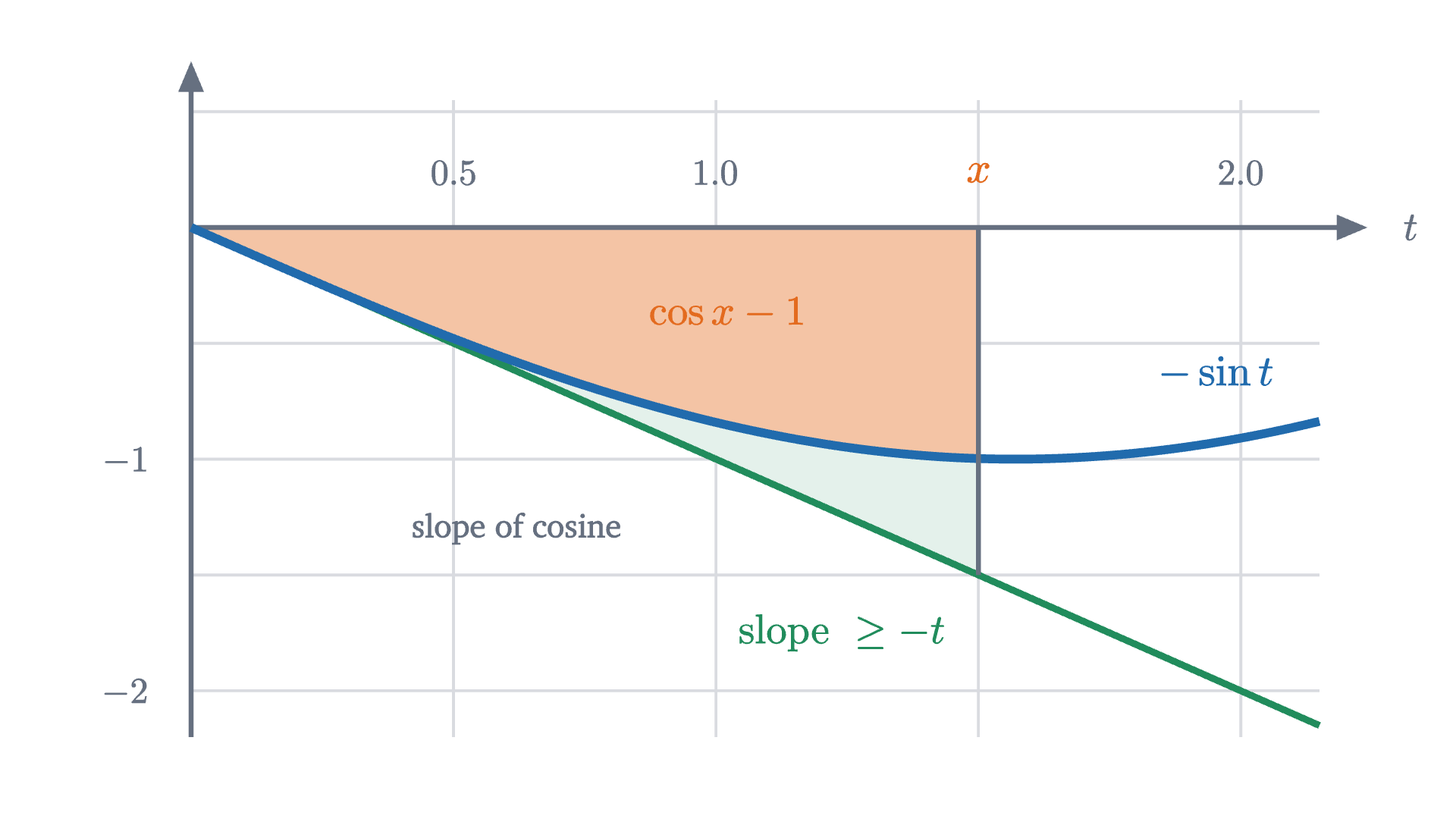
The slope of \cos t is -\sin t (blue). Because that slope starts at 0 and changes at a rate of at most 1, it stays above the line -t (green). The total change in cosine from 0 to x is the orange area, which therefore fits inside a triangle of area x^2/2. — The slope of $\cos t$ is $-\sin t$ (blue). Because that slope starts at 0 and changes at a rate of at most 1, it stays above the line $-t$ (green). The total change in cosine from 0 to $x$ is the orange area, which therefore fits inside a triangle of area $x^2/2$.

So $\cos x \ge 1 - \frac{x^2}{2}$, and the same reasoning with the upper line gives $\cos x \le 1 + \frac{x^2}{2}$. A bound of 1 on the second derivative became a bound of $t$ on the first derivative and then a bound of $\frac{x^2}{2}$ on the function. Each step is an integration, and each integration raises the power by one and divides by the new exponent: $1 \to t \to \frac{t^2}{2} \to \frac{t^3}{2 \cdot 3} \to \frac{t^4}{2 \cdot 3 \cdot 4}$. The factorials are back, for the same reason as before, run in reverse.

Pause and try

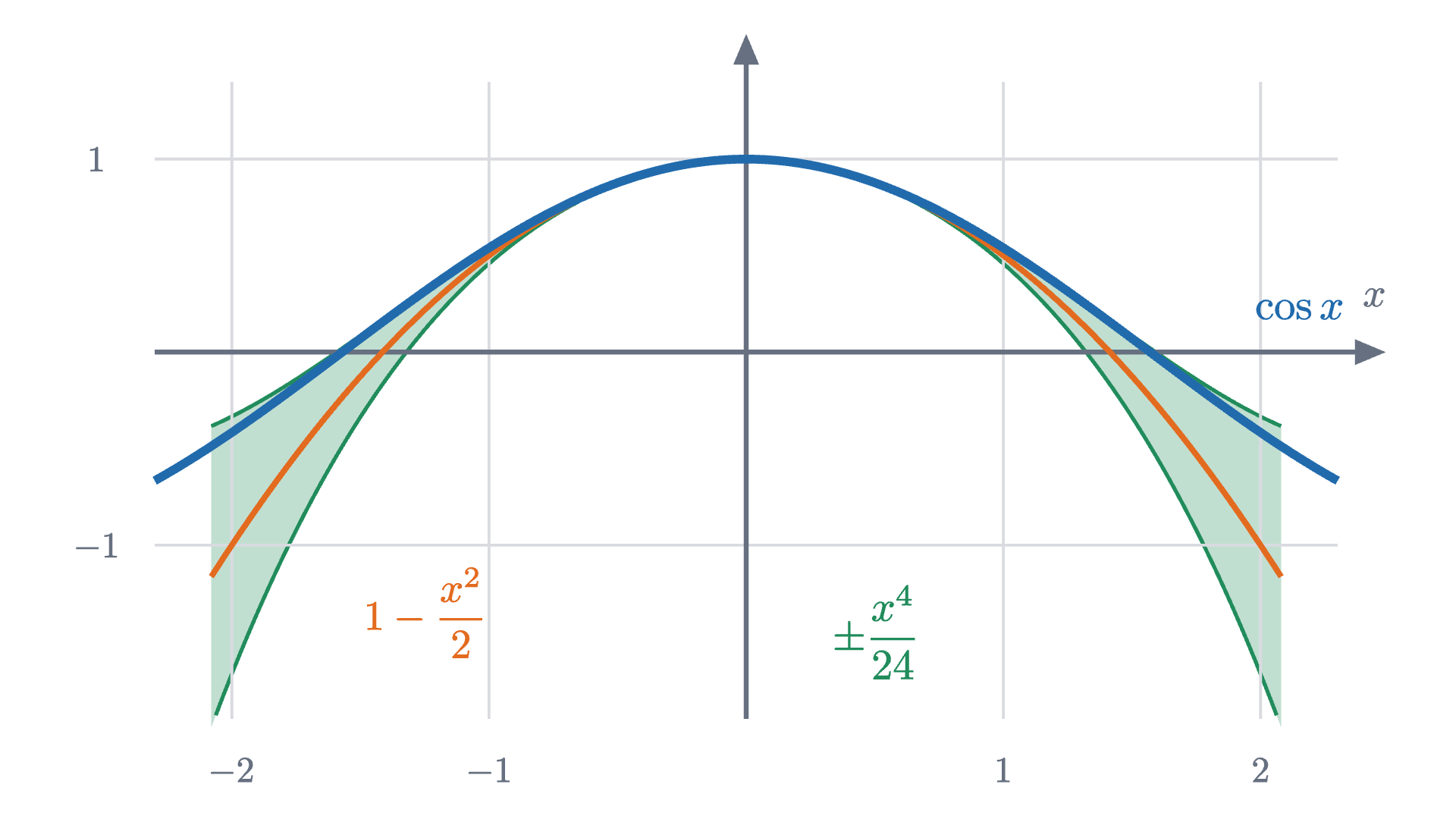
The fourth derivative of cosine is also at most 1 in size. Carry the chain four steps, applied to the difference between $\cos x$ and $1 - \frac{x^2}{2}$ (whose value and first three derivatives at 0 are all 0). What bound do you get for $\left|\cos(0.3) - 0.955\right|$, and how does it compare with the actual error in the table?

Show answerHide answer

The difference $g(x) = \cos x - \left(1 - \frac{x^2}{2}\right)$ has fourth derivative $\cos x$, since the polynomial’s fourth derivative is 0. Four integrations starting from $|g''''| \le 1$ give $|g'''| \le t$, $|g''| \le \frac{t^2}{2}$, $|g'| \le \frac{t^3}{6}$ and $|g(x)| \le \frac{x^4}{24}$. At $x = 0.3$ this is $\frac{0.0081}{24} = 0.0003375$. The actual error is $0.000336$. The guarantee is almost exactly attained, and we found it without knowing the answer.

The guarantee as a picture. With the bound |\cos''''| \le 1, the graph of cosine (blue) cannot leave the green funnel between 1 - \frac{x^2}{2} - \frac{x^4}{24} and 1 - \frac{x^2}{2} + \frac{x^4}{24}. The funnel is too thin to see near 0 and opens as x^4. — The guarantee as a picture. With the bound $|\cos''''| \le 1$, the graph of cosine (blue) cannot leave the green funnel between $1 - \frac{x^2}{2} - \frac{x^4}{24}$ and $1 - \frac{x^2}{2} + \frac{x^4}{24}$. The funnel is too thin to see near 0 and opens as $x^4$.

Taylor’s theorem

The argument for cosine used nothing about cosine except a bound on a derivative, so it should work for any function. The general statement keeps exact track of the error and not only of its size. Recall the fundamental theorem of calculus: if $F'$ is continuous on an interval containing $a$ and $x$, then $\int_a^x F'(t)\,dt = F(x) - F(a)$. This holds for $x < a$ as well, under the convention that an integral with its limits written backwards is the negative of the integral with them in order.

The hypotheses are what the cosine argument needed: enough derivatives to form $P_n$, and one more, $f^{(n+1)}$, to control what $P_n$ leaves out. $M$ is the speed limit. The power $|x - a|^{n+1}$ and the factorial are the result of integrating $n + 1$ times.

Proof

Fix $x$ and argue by induction on $n$.

The case $n = 0$. Here $P_0(x) = f(a)$ and the claim is $f(x) = f(a) + \int_a^x f'(t)\,dt$, which is the fundamental theorem.

From $n - 1$ to $n$ (for $n \ge 1$). Assume $f(x) = P_{n-1}(x) + R_{n-1}(x)$. Consider, as a function of $t$,

g(t) = \frac{(x - t)^n}{n!}\,f^{(n)}(t).

By the product rule, and the chain rule for $(x - t)^n$, whose derivative in $t$ is $-n(x-t)^{n-1}$,

g'(t) = -\frac{(x-t)^{n-1}}{(n-1)!}\,f^{(n)}(t) + \frac{(x-t)^n}{n!}\,f^{(n+1)}(t).

Both terms on the right are continuous in $t$, because $f^{(n)}$ and $f^{(n+1)}$ are, so $g'$ is continuous and we may integrate both sides from $a$ to $x$. On the left the fundamental theorem gives $g(x) - g(a) = 0 - \frac{(x-a)^n}{n!}f^{(n)}(a)$. On the right the two integrals are $-R_{n-1}(x)$ and $R_n(x)$. So

R_{n-1}(x) = \frac{f^{(n)}(a)}{n!}(x - a)^n + R_n(x).

The first term on the right is exactly the term that turns $P_{n-1}$ into $P_n$. Hence $f(x) = P_{n-1}(x) + R_{n-1}(x) = P_n(x) + R_n(x)$.

The bound. Suppose $x > a$. For $t$ in $[a, x]$ the factor $(x-t)^n$ is nonnegative, so the integrand lies between $-M(x-t)^n$ and $M(x-t)^n$, and so does its integral:

|R_n(x)| \le \frac{M}{n!}\int_a^x (x-t)^n\,dt = \frac{M}{n!} \cdot \frac{(x-a)^{n+1}}{n+1} = \frac{M(x-a)^{n+1}}{(n+1)!}.

For $x < a$ the same computation with $|x - t| = t - x$ gives $\frac{M(a - x)^{n+1}}{(n+1)!}$.

The induction step is the cosine argument in general form: each pass peels one more term off the remainder and leaves an integral with one more power of $(x - t)$ and one more derivative of $f$. The proof keeps every step an equation by carrying the exact integral along, and takes absolute values only at the end, so it also yields a formula for the error and not only a bound.

What convergence means

The theorem measures the error of one polynomial. The table suggested more: that by raising the degree we can get as close to $\cos(0.3)$ as we like.

An infinite sum is by definition a limit of finite sums, so the sentence “$\cos x = 1 - \frac{x^2}{2!} + \frac{x^4}{4!} - \cdots$” is a claim about a limit, to be proved separately for each $x$. The claim has two parts that can fail independently: that the numbers $P_n(x)$ approach something, and that the something is $f(x)$.

Proof

Fix $x$ and take $a = 0$. Every derivative of $\cos$ and of $\sin$ is one of $\pm\sin$, $\pm\cos$, so Taylor’s theorem applies with $M = 1$ for every $n$. For $e^x$ we use the fact that it is its own derivative, so $f^{(n+1)}(t) = e^t \le e^{|x|}$ for $t$ between 0 and $x$, and $M = e^{|x|}$ works for every $n$. In all three cases

|R_n(x)| \le M\,\frac{|x|^{n+1}}{(n+1)!}

with $M$ not depending on $n$. It remains to show that $\frac{|x|^m}{m!} \to 0$ as $m \to \infty$. Choose a whole number $N \ge 2|x|$. For $m > N$,

\frac{|x|^m}{m!} = \frac{|x|^N}{N!} \cdot \frac{|x|}{N+1} \cdot \frac{|x|}{N+2} \cdots \frac{|x|}{m} \le \frac{|x|^N}{N!}\left(\frac12\right)^{m-N},

because each of the $m - N$ later factors is at most $\frac12$. The right side is a fixed number times a power of $\frac12$, so it tends to 0.

That $e^x$ is its own derivative is the property that singles out the number $e$ among bases; we are quoting it, not proving it here.

The last step of the proof deserves a picture, because for large $x$ the terms of the series first grow.

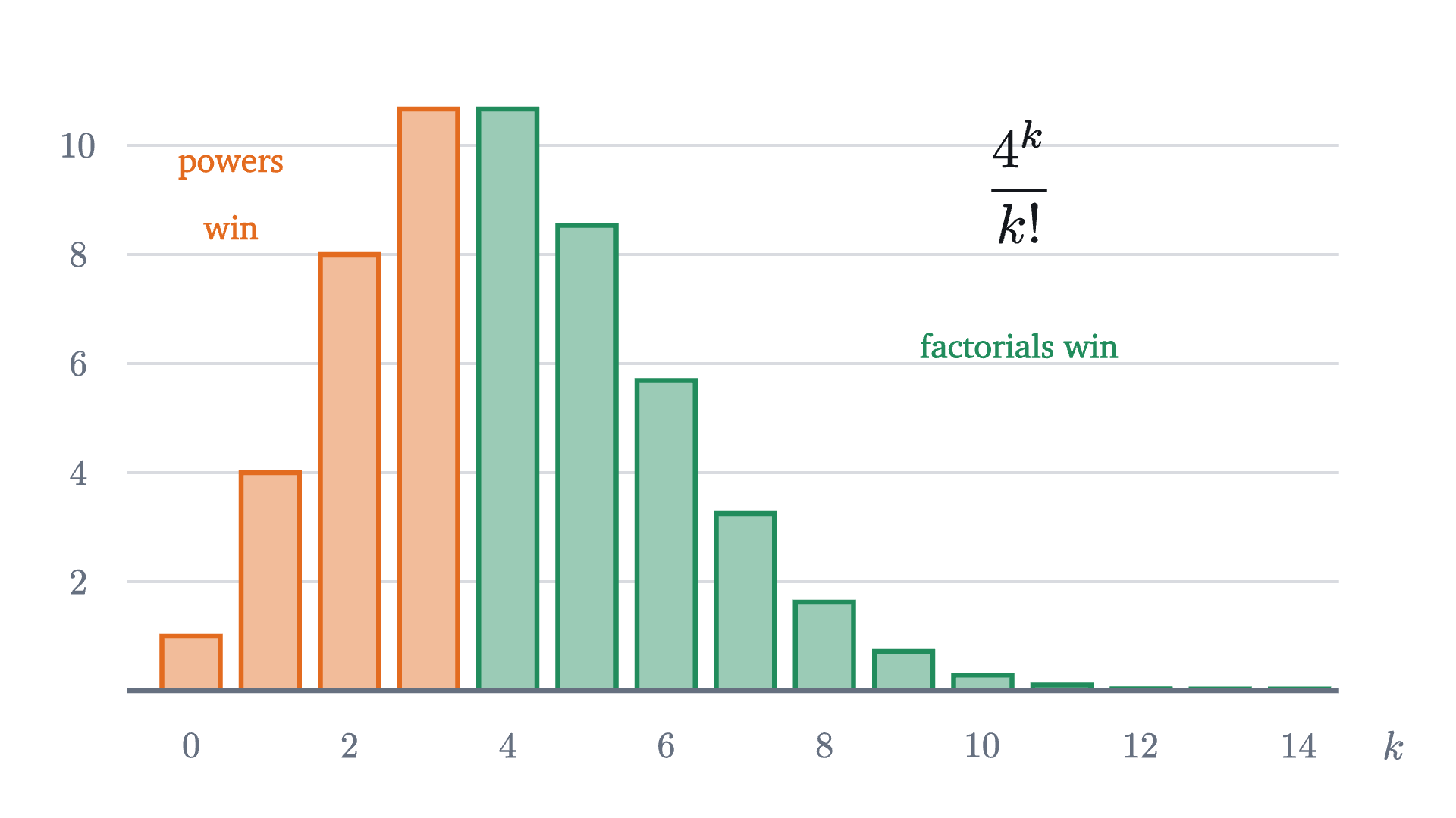
The sizes of the terms 4^k/k! of the series for e^4. Each bar is the previous one times 4/k, so the bars rise up to k = 3 (orange), hold level at k = 4 and fall from then on (green). Past k = 8 every bar is less than half the one before it. — The sizes of the terms $4^k/k!$ of the series for $e^4$. Each bar is the previous one times $4/k$, so the bars rise up to $k = 3$ (orange), hold level at $k = 4$ and fall from then on (green). Past $k = 8$ every bar is less than half the one before it.

A power $x^k$ gains the same factor $x$ at each step, while $k!$ gains a factor $k$ that keeps growing. Sooner or later the factorial wins, whatever $x$ is. So for these three functions a calculator can reach any accuracy at any $x$ by taking enough terms, though for large $x$ it may need many.

Where it fails

The proof for $\cos$, $\sin$ and $e^x$ leaned on one thing: a bound $M$ on the derivatives that does not grow with $n$. Here is a function without one. Let

f(x) = \frac{1}{1 - x}, \qquad x \ne 1.

By the chain rule its derivatives are $f'(x) = \frac{1}{(1-x)^2}$, $f''(x) = \frac{2}{(1-x)^3}$, and in general $f^{(k)}(x) = \frac{k!}{(1-x)^{k+1}}$. At 0 the $k$-th derivative is $k!$, which the $k!$ in the Taylor coefficient cancels. The Taylor series about 0 is

1 + x + x^2 + x^3 + \cdots

Pause and try

Compute the Taylor polynomials $P_0, P_1, P_2, P_3, P_4$ of $\frac{1}{1-x}$ at $x = \frac12$, where the function equals 2, and at $x = 2$, where it equals $-1$. What happens in each case?

Show answerHide answer

At $x = \frac12$: $1,\ 1.5,\ 1.75,\ 1.875,\ 1.9375$. Each term halves the remaining distance to 2. At $x = 2$: $1,\ 3,\ 7,\ 15,\ 31$. The values run away from $-1$ and do not approach anything. More terms make the approximation worse.

The function $\frac{1}{1-x}$ (blue) and its Taylor polynomials $1 + x + \cdots + x^n$ about 0 (orange) for $n = 1$ to $14$. Inside the green strip $-1 < x < 1$ the polynomials settle onto the curve. Outside it they swing further away with every added term.

Monocurl source

let fw = Frame(-2.5, 2.5, -3.2, 7.2, [0.1, 0.05, 0], 6.5, 3.5)
mesh strip = Region([at(fw, -1, -3.2), at(fw, 1, -3.2), at(fw, 1, 7.2), at(fw, -1, 7.2)], tint(LEAF, 0.14))
mesh plot = Plot(fw, [-2, -1, 1, 2], [-2, 2, 4, 6])
mesh walls = [
    stroke{LEAF, 2.5} dashed{[0.12, 0.08]} Line(at(fw, -1, -3.2), at(fw, -1, 7.2)),
    stroke{ROSE, 2.5} dashed{[0.12, 0.08]} Line(at(fw, 1, -3.2), at(fw, 1, 7.2))
]
mesh curve = [
    Clip(fw, |x| 1 / (1 - x), -2.5, 0.99, AZURE, 4.5),
    Clip(fw, |x| 1 / (1 - x), 1.01, 2.5, AZURE, 4.5)
]
mesh poly = GeoPoly(fw, 1)
mesh tag = Tag([-2.15, 2.02, 0], "degree 1", EMBER)

slide "wall"
    play Wait(0.6)
    for (n in range(2, 15)) {
        poly = GeoPoly(fw, n)
        tag = Tag([-2.15, 2.02, 0], str_join(["degree ", to_string(n)]), EMBER)
        play [Fade(0.3, [&poly]), Set([&tag])]
        play Wait(0.3)
    }
    play Wait(1.6)

Uses the shared definitions for this lesson's figures.

For this function we do not need the integral to find the remainder. Multiplying out, $(1 - x)(1 + x + \cdots + x^n) = 1 - x^{n+1}$, so for $x \ne 1$

\frac{1}{1-x} - \left(1 + x + \cdots + x^n\right) = \frac{x^{n+1}}{1 - x}.

This is $R_n(x)$ exactly. It tends to 0 when $|x| < 1$, and when $|x| \ge 1$ it does not, because $|x|^{n+1}$ does not shrink. So the series converges to $f(x)$ on the interval $-1 < x < 1$ and nowhere else.

The barrier on the right is understandable: $f$ has no value at $x = 1$, and its graph runs off to infinity there. The barrier on the left is the surprising one. At $x = -1$ the function is perfectly well behaved, $f(-1) = \frac12$, yet the series gives $1 - 1 + 1 - 1 + \cdots$, whose partial sums alternate between 1 and 0 forever. A series in powers of $x$ cannot tell $x$ from $-x$ as far as size is concerned: its terms have size $|x|^k$ either way. The trouble at distance 1 on one side shuts the series down at distance 1 on every side.

That behavior is general. It is a theorem of analysis, which we state without proof, that every series $\sum c_k(x-a)^k$ has a radius of convergence $R$ (possibly 0 or infinite): it converges when $|x - a| < R$ and diverges when $|x - a| > R$. For $\cos$, $\sin$ and $e^x$ about any point, $R$ is infinite. For $\frac{1}{1-x}$ about 0, $R = 1$.

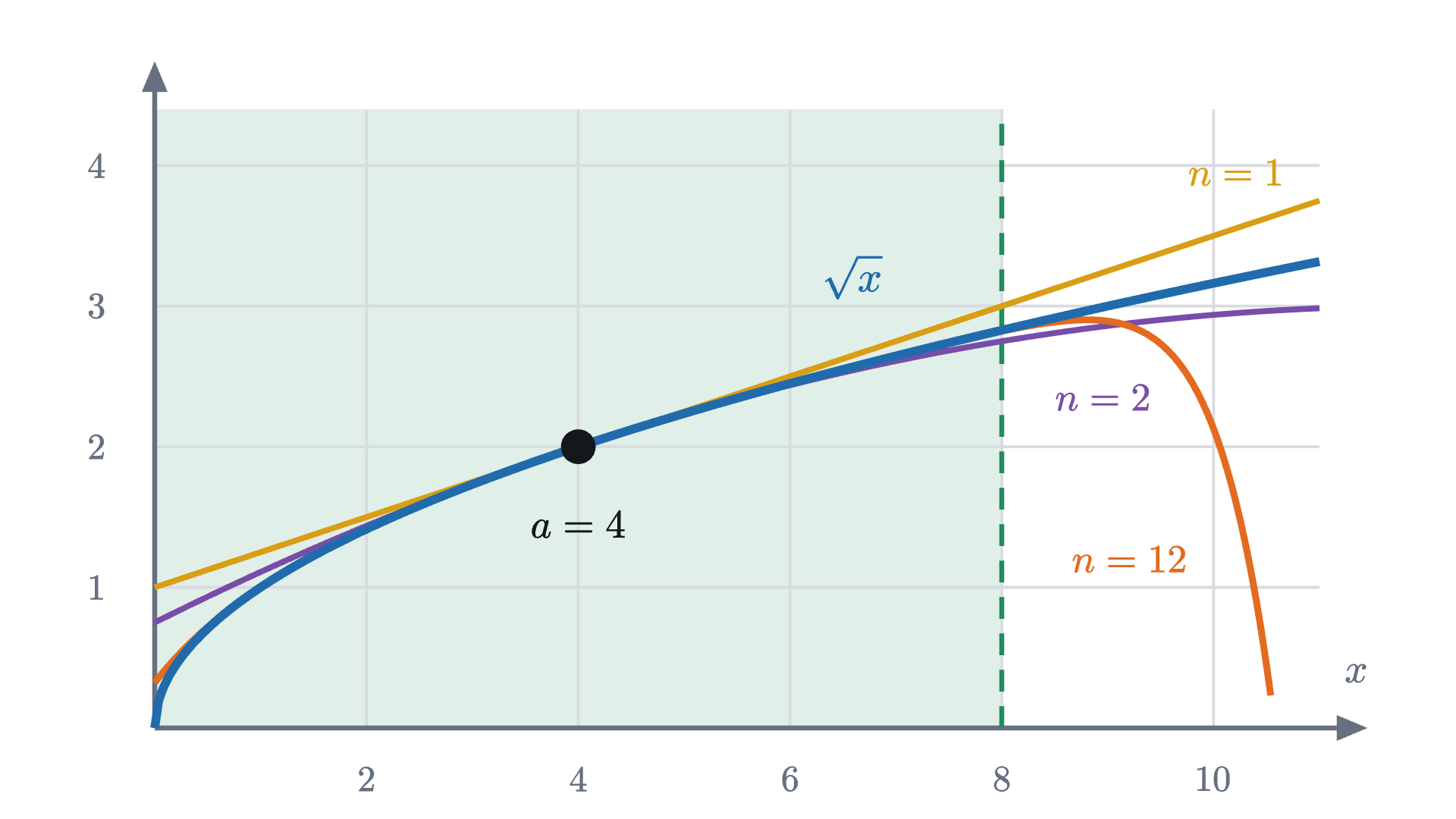
Taylor’s theorem has not failed here. It is still true for every $n$ and every $x < 1$. What fails is the bound’s usefulness: on the interval from 0 to $x$ the derivative $f^{(n+1)}(t) = \frac{(n+1)!}{(1-t)^{n+2}}$ has a maximum $M$ of at least $(n+1)!$, its value at $t = 0$. The factorial in the bound, which was supposed to beat the power, is cancelled, and what is left is at least $|x|^{n+1}$.

There is a second way to fail, and it is stranger. The function defined by $f(x) = e^{-1/x^2}$ for $x \ne 0$ and $f(0) = 0$ has derivatives of all orders at 0, and every one of them equals 0 (an example that goes back to Cauchy in the 1820s; the verification is a standard exercise). Its Taylor series about 0 is $0 + 0 + 0 + \cdots$, which converges for every $x$, to 0. But $f(x) > 0$ for $x \ne 0$. The series converges, and to the wrong function. Matching every derivative at one point does not by itself pin a function down; an estimate of the remainder is what does.

Worked examples

Worked example

Estimate $\sqrt{4.1}$ and bound the error.

We want a center where the function and its derivatives are easy, and $a = 4$ is close to $4.1$. With $f(x) = x^{1/2}$ the power rule gives

f'(x) = \tfrac12 x^{-1/2}, \qquad f''(x) = -\tfrac14 x^{-3/2}, \qquad f'''(x) = \tfrac38 x^{-5/2}.

At $a = 4$: $f(4) = 2$, $f'(4) = \frac14$, $f''(4) = -\frac{1}{32}$. So

P_2(x) = 2 + \frac14(x - 4) - \frac{1}{64}(x-4)^2, \qquad P_2(4.1) = 2 + 0.025 - 0.00015625 = 2.02484375.

For the error we need a bound on $f'''$ between 4 and 4.1. Since $x^{-5/2}$ decreases as $x$ grows, its largest value there is at $x = 4$: $M = \frac38 \cdot \frac{1}{32} = \frac{3}{256}$. Taylor’s theorem with $n = 2$ gives

|R_2(4.1)| \le \frac{3}{256} \cdot \frac{0.1^3}{3!} \approx 0.00000195.

So $\sqrt{4.1}$ is within $0.000002$ of $2.02484375$. (A calculator gives $2.0248457$, which is $0.0000019$ away.)

\sqrt{x} (blue) and its Taylor polynomials about a = 4 of degree 1, 2 and 12. The square root has no derivative at x = 0, a distance 4 from the center, and the radius of convergence is 4: the degree-12 polynomial follows the curve across the green strip from 0 to 8 and leaves it just beyond 8. — $\sqrt{x}$ (blue) and its Taylor polynomials about $a = 4$ of degree 1, 2 and 12. The square root has no derivative at $x = 0$, a distance 4 from the center, and the radius of convergence is 4: the degree-12 polynomial follows the curve across the green strip from 0 to 8 and leaves it just beyond 8.

Check yourself

The degree-2 Taylor polynomial of $\cos x$ about 0 is used to estimate $\cos(0.1)$. Which statement is correct?

Looking back, finding the polynomials took one differentiation per coefficient. The hard part was knowing how far to trust them, and the answer came from turning a bound on the next derivative into a bound on the error by repeated integration. That idea, a local description plus a controlled remainder, is how most functions are computed in practice and how most approximations in physics are justified.

Recap

The Taylor polynomial $P_n(x) = \sum_{k=0}^n \frac{f^{(k)}(a)}{k!}(x-a)^k$ matches the value and first $n$ derivatives of $f$ at $a$. The $k!$ is there because $x^k$ differentiated $k$ times is $k!$.
Taylor’s theorem: $f(x) - P_n(x) = \frac{1}{n!}\int_a^x (x-t)^n f^{(n+1)}(t)\,dt$, and this is at most $\frac{M|x-a|^{n+1}}{(n+1)!}$ in size when $|f^{(n+1)}| \le M$ between $a$ and $x$.
The Taylor series converges to $f(x)$ at $x$ exactly when $R_n(x) \to 0$. For $\cos$, $\sin$ and $e^x$ this holds for every $x$, because their derivatives stay bounded while $(n+1)!$ outgrows $|x|^{n+1}$.
$\frac{1}{1-x} = 1 + x + x^2 + \cdots$ only for $|x| < 1$. A series converges inside its radius of convergence and diverges beyond it.
A Taylor series can also converge to the wrong function ($e^{-1/x^2}$). Agreement of derivatives at one point is not enough; the remainder must be shown to vanish.

Problems

The first three repeat the lesson’s computations, the next four ask you to combine them with a bound or an argument, and the last one reaches a famous series.

Problem 1

Use the degree-3 Taylor polynomial of $\sin x$ about 0 to estimate $\sin(0.2)$, and bound the error. (Notice that $P_3 = P_4$.)

Show solutionHide solution

$P_3(x) = x - \frac{x^3}{6}$, so $P_3(0.2) = 0.2 - \frac{0.008}{6} = 0.198667$ to six places. The $x^4$ coefficient of sine is 0, so this is also $P_4(0.2)$, and the theorem with $n = 4$, $M = 1$ gives $|R_4| \le \frac{0.2^5}{5!} = \frac{0.00032}{120} \approx 0.0000027$. (The true value is $0.1986693$.)

Problem 2

Write down the degree-4 Taylor polynomial of $e^x$ about 0, use it to estimate $e^{0.1}$, and bound the error, using $e^{0.1} < 3$.

Show solutionHide solution

$P_4(x) = 1 + x + \frac{x^2}{2} + \frac{x^3}{6} + \frac{x^4}{24}$. At $0.1$: $1 + 0.1 + 0.005 + 0.000166667 + 0.000004167 = 1.105170833$. The fifth derivative $e^t$ is at most $e^{0.1} < 3$ on $[0, 0.1]$, so $|R_4| \le \frac{3 \times 0.1^5}{5!} = \frac{0.00003}{120} = 2.5 \times 10^{-7}$. (The true value is $1.105170918$, an error of about $8.5 \times 10^{-8}$.)

Problem 3

Find the Taylor polynomial of every degree for $f(x) = x^3$ about $a = 1$. What is the remainder $R_3$?

Show solutionHide solution

$f(1) = 1$, $f'(x) = 3x^2$ so $f'(1) = 3$, $f''(x) = 6x$ so $f''(1) = 6$, $f'''(x) = 6$, and all later derivatives are 0. So $P_0 = 1$, $P_1 = 1 + 3(x-1)$, $P_2 = 1 + 3(x-1) + 3(x-1)^2$, and $P_n = 1 + 3(x-1) + 3(x-1)^2 + (x-1)^3$ for every $n \ge 3$. Since $f^{(4)} = 0$, the integral form gives $R_3(x) = 0$: the polynomial $P_3$ equals $x^3$ exactly. Expanding confirms it: with $u = x - 1$, $(1 + u)^3 = 1 + 3u + 3u^2 + u^3$. A Taylor polynomial of a polynomial is the same polynomial rewritten in powers of $(x - a)$.

Problem 4

Find the Taylor series of $f(x) = \frac{1}{x}$ about $a = 1$. For which $x$ does it converge to $\frac1x$? Explain the answer in terms of the graph.

Show solutionHide solution

$f'(x) = -x^{-2}$, $f''(x) = 2x^{-3}$, $f'''(x) = -6x^{-4}$, and in general $f^{(k)}(x) = (-1)^k k!\,x^{-(k+1)}$, so $\frac{f^{(k)}(1)}{k!} = (-1)^k$. The series is $\sum (-1)^k (x-1)^k = 1 - (x-1) + (x-1)^2 - \cdots$. Put $u = 1 - x$: this is $1 + u + u^2 + \cdots$, and $\frac1x = \frac{1}{1 - u}$. By the lesson’s computation the remainder is $\frac{u^{n+1}}{1-u}$, which tends to 0 exactly when $|u| < 1$, that is, $0 < x < 2$. The radius of convergence is 1, the distance from the center $a = 1$ to the point $x = 0$ where $\frac1x$ has no value. The series stops at $x = 2$ as well, where the function is harmless, for the same reason as in the lesson.

Problem 5

How many nonzero terms of the cosine series guarantee $\cos(1)$ to within $10^{-8}$?

Show solutionHide solution

With $M = 1$ and $x = 1$, $|R_n(1)| \le \frac{1}{(n+1)!}$. We need $(n+1)! \ge 10^8$. Since $11! = 39{,}916{,}800$ and $12! = 479{,}001{,}600$, we need $n + 1 = 12$, so $n = 11$. Because cosine has no odd powers, $P_{11} = P_{10}$, which has the six nonzero terms $1 - \frac{1}{2!} + \frac{1}{4!} - \frac{1}{6!} + \frac{1}{8!} - \frac{1}{10!} = 0.5403023038$. (The true value is $0.5403023059$, and the error $2.1 \times 10^{-9}$ equals the bound $\frac{1}{12!}$ to two digits.)

Problem 6

Use the integral form of the remainder with $n = 1$ to prove that $\cos x \ge 1 - \frac{x^2}{2}$ for every real $x$.

Show solutionHide solution

With $f = \cos$, $a = 0$, $n = 1$: $P_1(x) = 1$ and $f'' = -\cos$, so $\cos x = 1 + \int_0^x (x - t)(-\cos t)\,dt$. Suppose $x \ge 0$. For $t$ in $[0, x]$ we have $x - t \ge 0$ and $-\cos t \ge -1$, so the integrand is at least $-(x - t)$, and

\cos x \ge 1 - \int_0^x (x - t)\,dt = 1 - \frac{x^2}{2}.

For $x < 0$, use that both sides are unchanged when $x$ is replaced by $-x$: $\cos(-x) = \cos x$ and $(-x)^2 = x^2$. So the inequality for $-x > 0$ is the inequality for $x$.

Problem 7

Use Taylor’s theorem to show that $\left|\frac{\sin x}{x} - 1\right| \le \frac{x^2}{6}$ for all $x \ne 0$, and deduce $\lim_{x \to 0} \frac{\sin x}{x} = 1$.

Show solutionHide solution

For sine about 0, $P_1(x) = x$ and the $x^2$ coefficient is 0, so $P_2(x) = x$ too. The theorem with $n = 2$ and $M = 1$ (the third derivative is $-\cos$) gives $|\sin x - x| \le \frac{|x|^3}{6}$. Dividing by $|x| > 0$: $\left|\frac{\sin x}{x} - 1\right| \le \frac{x^2}{6}$. Given $\varepsilon > 0$, take $\delta = \sqrt{6\varepsilon}$; then $0 < |x| < \delta$ implies $\frac{x^2}{6} < \varepsilon$. This is the $\varepsilon$–$\delta$ definition of the limit. (There is no circularity as long as the derivative of sine was obtained geometrically, as in the lesson on the derivative of sine.)

Problem 8

The derivative of $\arctan x$ is $\frac{1}{1 + x^2}$, and $\arctan 1 = \frac{\pi}{4}$. (a) Replace $x$ by $-t^2$ in the identity $\frac{1}{1-x} = 1 + x + \cdots + x^n + \frac{x^{n+1}}{1-x}$. (b) Integrate the result from 0 to 1 and show that the last term contributes at most $\frac{1}{2n+3}$ in size. (c) Conclude that $\frac{\pi}{4} = 1 - \frac13 + \frac15 - \frac17 + \cdots$.

Show solutionHide solution

(a) $\frac{1}{1 + t^2} = 1 - t^2 + t^4 - \cdots + (-1)^n t^{2n} + \frac{(-1)^{n+1} t^{2n+2}}{1 + t^2}$, valid for every real $t$ since $-t^2 \ne 1$.

(b) By the fundamental theorem, $\int_0^1 \frac{dt}{1+t^2} = \arctan 1 - \arctan 0 = \frac{\pi}{4}$, and $\int_0^1 t^{2k}\,dt = \frac{1}{2k+1}$. So

\frac{\pi}{4} = 1 - \frac13 + \frac15 - \cdots + \frac{(-1)^n}{2n+1} + E_n, \qquad E_n = (-1)^{n+1}\int_0^1 \frac{t^{2n+2}}{1+t^2}\,dt.

Since $0 \le \frac{t^{2n+2}}{1 + t^2} \le t^{2n+2}$ on $[0, 1]$, we get $|E_n| \le \int_0^1 t^{2n+2}\,dt = \frac{1}{2n+3}$.

(c) $\frac{1}{2n+3} \to 0$, so the partial sums converge to $\frac{\pi}{4}$. Notice where we are: the series $1 - t^2 + t^4 - \cdots$ has radius of convergence 1, and $t = 1$ is on the edge, where the series itself reads $1 - 1 + 1 - \cdots$ and diverges. We never used the infinite series at $t = 1$. We used a finite sum with an exact remainder and bounded the remainder after integrating, which is the method of this whole lesson. The convergence is slow, with an error of order $\frac1n$, so a thousand terms give about three digits of $\pi$.

Shared definitions used by this lesson's figures

# house kit: prepended to every essay figure after the std imports

# palette. AZURE and EMBER are the two actors, LEAF marks an answer, ROSE a problem
let PAPER = [1, 1, 1, 1]
let INK = [0.08, 0.09, 0.11, 1]
let SLATE = [0.40, 0.44, 0.50, 1]
let MIST = [0.85, 0.86, 0.88, 1]
let AZURE = [0.13, 0.42, 0.68, 1]
let EMBER = [0.89, 0.42, 0.12, 1]
let LEAF = [0.13, 0.55, 0.36, 1]
let ROSE = [0.78, 0.22, 0.24, 1]
let PLUM = [0.47, 0.30, 0.66, 1]
let GOLD = [0.85, 0.62, 0.08, 1]

background = PAPER

# an opaque pastel of col; use for fills so overlaps do not darken
let tint = |col, amount = 0.18| [
    1 - (1 - col[0]) * amount,
    1 - (1 - col[1]) * amount,
    1 - (1 - col[2]) * amount,
    1
]

# text: Cap for labels, Note for quiet labels, Math for typeset maths
let Cap = |txt, size = 0.75, col = INK| color{col} Text(txt, size, "Charter")
let Note = |txt, size = 0.65| color{SLATE} Text(txt, size, "Charter")
let Math = |tex, size = 0.9, col = INK| color{col} Tex(tex, size)

# a paper rectangle to sit behind text that crosses lines
let Plate = |pos, size| center{pos} fill{PAPER} stroke{alpha{0} PAPER, 0} Rect(size)

# shapes with fill and stroke both set, so no stray black appears
let Pt = |pos, col = INK, r = 0.075| center{pos} fill{col} stroke{col, 1} Circle(r, 48)
let Ring = |pos, col = INK, r = 0.1, w = 3| center{pos} fill{PAPER} stroke{col, w} Circle(r, 48)
let Seg = |a, b, col = INK, w = 3| stroke{col, w} Line(a, b)
let Path = |pts, col = INK, w = 3| stroke{col, w} Polyline(pts)
let Region = |pts, col| fill{col} stroke{alpha{0} col, 0} Polygon(pts)
let Outline = |pts, col = INK, w = 3| fill{alpha{0} PAPER} stroke{col, w} Polygon(pts)
let Shape = |pts, col, amount = 0.18, w = 3| fill{tint(col, amount)} stroke{col, w} Polygon(pts)
let Disc = |pos, r, col, amount = 0.18, w = 3| center{pos} fill{tint(col, amount)} stroke{col, w} Circle(r, 96)
let Box = |pos, size, col, amount = 0.18, w = 3| center{pos} fill{tint(col, amount)} stroke{col, w} Rect(size)
# a line from a to b ending in a small solid arrowhead
let Tip = |a, b, col = INK, w = 3, head = 0.17| {
    let d = normalize([b[0] - a[0], b[1] - a[1], 0])
    let n = [-d[1], d[0], 0]
    let base = [b[0] - d[0] * head, b[1] - d[1] * head, 0]
    return [
        stroke{col, w} Line(a, base),
        fill{col} stroke{col, 1} Polygon([
            b,
            [base[0] + n[0] * head * 0.42, base[1] + n[1] * head * 0.42, 0],
            [base[0] - n[0] * head * 0.42, base[1] - n[1] * head * 0.42, 0]
        ])
    ]
}

# plots. a frame is [x0, x1, y0, y1, centre, width, height]: a data window and the scene box it fills
let Frame = |x0, x1, y0, y1, c = [0, 0, 0], w = 6.4, h = 3.6| [x0, x1, y0, y1, c, w, h]
let fx = |fr, x| fr[4][0] + (x - (fr[0] + fr[1]) / 2) * fr[5] / (fr[1] - fr[0])
let fy = |fr, y| fr[4][1] + (y - (fr[2] + fr[3]) / 2) * fr[6] / (fr[3] - fr[2])
let at = |fr, x, y| [fx(fr, x), fy(fr, y), 0]

# axes through the data origin (or the nearest edge of the window), with optional names
let Axes = |fr, x_name = "", y_name = "", col = SLATE| {
    let ox = clamp(fr[0], 0, fr[1])
    let oy = clamp(fr[2], 0, fr[3])
    var parts = [
        Tip(at(fr, fr[0], oy), [fx(fr, fr[1]) + 0.25, fy(fr, oy), 0], col, 2.5, 0.15),
        Tip(at(fr, ox, fr[2]), [fx(fr, ox), fy(fr, fr[3]) + 0.25, 0], col, 2.5, 0.15)
    ]
    if (x_name != "") {
        parts .= center{[fx(fr, fr[1]) + 0.5, fy(fr, oy), 0]} Math(x_name, 0.8, col)
    }
    if (y_name != "") {
        parts .= center{[fx(fr, ox), fy(fr, fr[3]) + 0.5, 0]} Math(y_name, 0.8, col)
    }
    return parts
}

# tick marks with numbers at the listed data values
let XTicks = |fr, xs, col = SLATE, places = 0| block {
    let oy = fy(fr, clamp(fr[2], 0, fr[3]))
    for (x in xs) {
        . Seg([fx(fr, x), oy - 0.07, 0], [fx(fr, x), oy + 0.07, 0], col, 2)
        . center{[fx(fr, x), oy - 0.33, 0]} Math(to_string(x, places), 0.72, col)
    }
}
let YTicks = |fr, ys, col = SLATE, places = 0| block {
    let ox = fx(fr, clamp(fr[0], 0, fr[1]))
    for (y in ys) {
        . Seg([ox - 0.07, fy(fr, y), 0], [ox + 0.07, fy(fr, y), 0], col, 2)
        . center{[ox - 0.36, fy(fr, y), 0]} Math(to_string(y, places), 0.72, col)
    }
}

# faint grid lines at the listed data values
let GridLines = |fr, xs, ys, col = MIST| block {
    for (x in xs) {
        . Seg(at(fr, x, fr[2]), at(fr, x, fr[3]), col, 1.5)
    }
    for (y in ys) {
        . Seg(at(fr, fr[0], y), at(fr, fr[1], y), col, 1.5)
    }
}

# the graph of f over [a, b], drawn in the frame. values are clamped to the window
let Graph = |fr, f, a, b, col = AZURE, w = 4, n = 160|
    stroke{col, w} Polyline(map(sample(a, b, n), |x| at(fr, x, clamp(fr[2], f(x), fr[3]))))

# the region between the graph of f and the x axis over [a, b]
let AreaUnder = |fr, f, a, b, col = AZURE, amount = 0.2, n = 80| {
    var pts = [at(fr, a, 0)]
    for (x in sample(a, b, n)) {
        pts .= at(fr, x, clamp(fr[2], f(x), fr[3]))
    }
    pts .= at(fr, b, 0)
    return fill{tint(col, amount)} stroke{alpha{0} col, 0} Polygon(pts)
}

# the Taylor polynomial of cos about 0, up to degree n
let cosP = |n, x| {
    var s = 1
    var term = 1
    for (k in range(1, n // 2 + 1)) {
        term = -term * x * x / ((2 * k - 1) * (2 * k))
        s = s + term
    }
    return s
}
# 1 + x + ... + x^n
let geoP = |n, x| {
    var s = 0
    var term = 1
    for (k in range(0, n + 1)) {
        s = s + term
        term = term * x
    }
    return s
}
# the graph of f over [a, b], keeping only the part inside the window
let Clip = |fr, f, a, b, col = AZURE, w = 4, n = 240| stroke{col, w} Polyline(filter(
    map(sample(a, b, n), |x| [fx(fr, x), fy(fr, f(x)), 0]),
    |p| p[1] >= fy(fr, fr[2]) and p[1] <= fy(fr, fr[3])
))
let CosPoly = |fr, n, col = EMBER, w = 4| Clip(fr, |x| cosP(n, x), fr[0], fr[1], col, w)
let GeoPoly = |fr, n, col = EMBER, w = 4| Clip(fr, |x| geoP(n, x), fr[0], fr[1], col, w)
# a plot with grid and axes; the numbers sit along the bottom and left edges, clear of the curves
let Plot = |fr, xs, ys| block {
    . GridLines(fr, xs, ys)
    . Axes(fr)
    . center{[fx(fr, fr[1]) + 0.2, fy(fr, clamp(fr[2], 0, fr[3])) + 0.3, 0]} Math("x", 0.8, SLATE)
    for (x in xs) {
        . center{[fx(fr, x), fy(fr, fr[2]) - 0.28, 0]} Math(to_string(x), 0.72, SLATE)
    }
    for (y in ys) {
        . center{[fx(fr, fr[0]) - 0.32, fy(fr, y), 0]} Math(to_string(y), 0.72, SLATE)
    }
}
let Tag = |pos, txt, col| center{pos} Cap(txt, 0.8, col)