Correlation and the line of best fit, derived

We derive the least-squares line, define the correlation r and prove it lies between -1 and 1, then explain regression to the mean and why r is not causation.

23 min·High school and early college·Updated October 2026

AssumesMean, median and standard deviation: what each one says What slope means, and why y = mx + b is a line

A simulation of 300 fathers and their adult sons, with heights that have correlation 0.5. Each blue dot is one pair. The orange dots are the average height of the sons for fathers of each height, and they follow the green line of best fit, which is flatter than the dashed line where a son is exactly as tall as his father.

Monocurl source

let R = corr(FATHERS, SONS)
let Cloud = |k| {
    let kk = to_int(floor(k + 0.0001))
    return map(filter(range(0, kk), |i| inside(FATHERS[i], SONS[i])), |i| Pt(at(ff, FATHERS[i], SONS[i]), alpha{0.7} AZURE, 0.045))
}
let StripMeans = block {
    for (lo in range(160, 192, 4)) {
        let sel = filter(range(0, NPAIR), |i| FATHERS[i] >= lo and FATHERS[i] < lo + 4)
        if (len(sel) >= 3) {
            . Pt(at(ff, lo + 2, mean(map(sel, |i| SONS[i]))), EMBER, 0.1)
        }
    }
}
mesh plot = [HeightPlot, SonName]
mesh cloud = Cloud(k: 0)
mesh lines = []
mesh strips = []
mesh legend = []

slide "pairs"
    play Wait(0.4)
    cloud.k = NPAIR
    play Lerp(4, [&cloud], linear)
    strips = StripMeans
    legend = [
        Pt([-2.2, 1.42, 0], EMBER, 0.1),
        center{[-0.45, 1.42, 0]} Cap("average son, by father's height", 0.7, EMBER)
    ]
    play Fade(0.8, [&strips, &legend])
    play Wait(0.6)
    lines = [SameLine, FitLine]
    legend = [
        legend,
        Seg([-2.4, 1.08, 0], [-2.0, 1.08, 0], LEAF, 4.5),
        center{[-1.15, 1.08, 0]} Cap("line of best fit", 0.7, LEAF),
        stroke{SLATE, 3} dashed{[0.14, 0.09]} Line([2.1, -0.62, 0], [2.5, -0.62, 0]),
        center{[2.25, -0.92, 0]} Cap("son = father", 0.7, SLATE),
        center{[2.25, -1.22, 0]} Math(str_join(["r = ", to_string(R, 2)]), 0.85, INK)
    ]
    play Fade(0.8, [&lines, &legend])
    play Wait(2.2)

Uses the shared definitions for this lesson's figures.

Tall fathers have tall sons, but not as tall as themselves: fathers who stand 184 cm have sons who average about 180. Short fathers have short sons, but not as short: fathers of 168 cm have sons who average about 172. Each generation, it seems, is pulled toward the middle.

Follow that thought and you reach an absurd conclusion. If every generation is closer to average than the one before, then after enough generations everyone should be nearly the same height. Yet the spread of heights among sons is the same as among fathers. Francis Galton noticed this pattern in the 1880s and called it “regression towards mediocrity”, which is where the word regression in statistics comes from. Resolving the paradox takes three things: what it means to fit a line to scattered data, a number that measures how tightly the data follow the line, and a hard look at what that number can and cannot tell you.

A cloud of points and a line through it

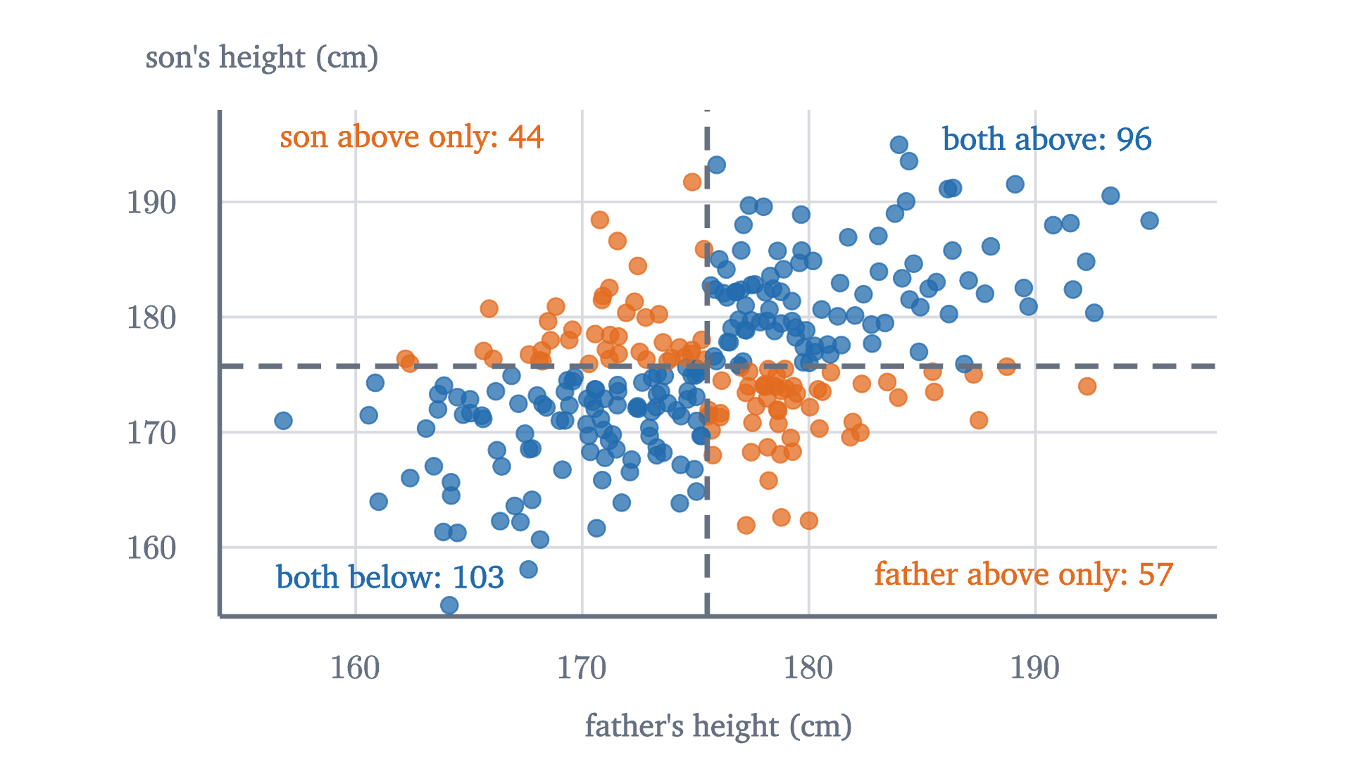
The figure above is a scatter plot: each dot stands for one father-son pair, placed at the father’s height horizontally and the son’s height vertically. The dots form a tilted cloud. Knowing the father’s height tells you something about the son’s, but far from everything.

To see how a line gets fitted to a cloud, we shrink the problem until it can be done by hand. Five students practice for $x = 1, 2, 3, 4, 5$ hours and score $y = 2, 4, 5, 4, 5$ on a test. A line $y = a + bx$ (intercept $a$, slope $b$) predicts a score for each student, and the prediction misses by $y_i - (a + bx_i)$. This vertical miss is called a residual.

What should “best” mean? We want all the residuals small at once, so we need one number that summarizes them. Their plain sum will not do: a line that misses one point by $+10$ and another by $-10$ would get a perfect total of zero. The same problem came up for the spread of data in the first lesson of this series, and we adopt the same repair. Square each residual, so that misses in both directions count against the line, and add.

Pause and try

An obvious candidate is the line through the first and last points, $(1, 2)$ and $(5, 5)$, which is $y = 1.25 + 0.75x$. Find its five residuals and the sum of their squares.

Show answerHide answer

The line predicts $2, 2.75, 3.5, 4.25, 5$. The residuals are $2 - 2 = 0$, $4 - 2.75 = 1.25$, $5 - 3.5 = 1.5$, $4 - 4.25 = -0.25$ and $5 - 5 = 0$. The squares are $0, 1.5625, 2.25, 0.0625, 0$, with sum $3.875$.

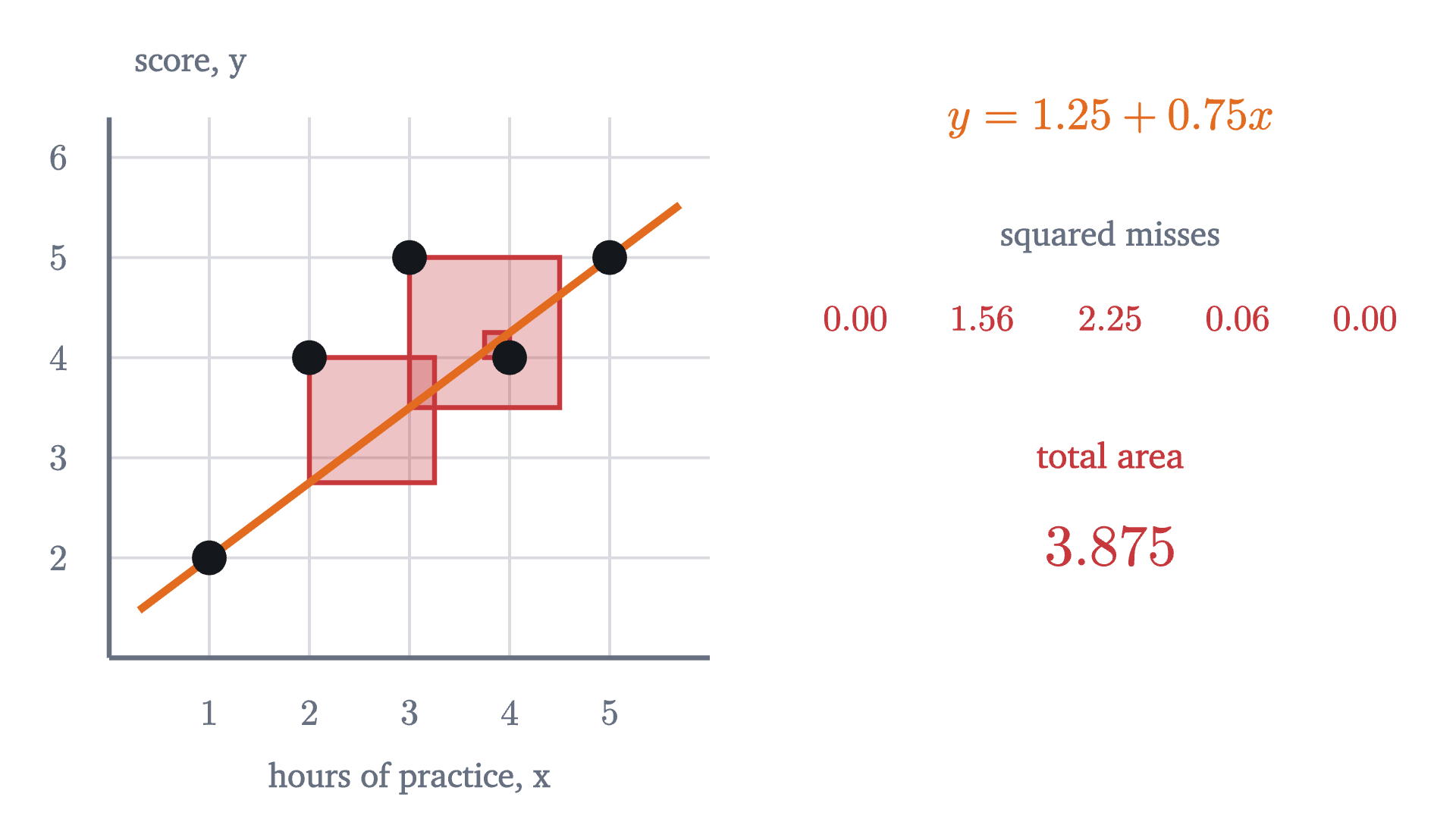
The five data points and the line through the first and last of them. Each residual is drawn as a square whose side is the vertical miss, so the line's total squared error, 3.875, is the total red area. Two of the residuals are zero and have no square. — The five data points and the line through the first and last of them. Each residual is drawn as a square whose side is the vertical miss, so the line’s total squared error, 3.875, is the total red area. Two of the residuals are zero and have no square.

That line runs too low through the middle: two points sit well above it, and none is far below. Tilting and shifting it should shrink the squares.

The line pivots and then slides, and the squares on the residuals grow and shrink with it. The total area starts at 6 for a flat line through the mean score, and is smallest, 2.4, when the slope is 0.6 and the line passes through the point of means $(3, 4)$.

Monocurl source

let Fit = |b, c| {
    let a = 4 + c - 3 * b
    return [
        Squares(fp, a, b),
        LineOn(fp, a, b, EMBER),
        Dots(fp),
        center{[2.1, 1.3, 0]} scale{1.15} color{EMBER} Number(b, 2),
        center{[2.1, 0.3, 0]} scale{1.15} color{EMBER} Number(4 + c, 2),
        center{[2.1, -0.95, 0]} scale{1.5} color{ROSE} Number(sq_total(a, b), 2)
    ]
}
mesh plot = [PointPlot(fp), PointNames(fp)]
mesh side = [
    center{[2.1, 1.72, 0]} Note("slope b", 0.74),
    center{[2.1, 0.72, 0]} Note("height of the line at x = 3", 0.74),
    center{[2.1, -0.4, 0]} Cap("total area of the squares", 0.76, ROSE)
]
mesh fit = Fit(b: 0, c: 0)

slide "wobble"
    play Wait(0.8)
    fit.b = 1
    play Lerp(2.2, [&fit])
    fit.b = 0.6
    play Lerp(1.6, [&fit])
    play Wait(0.5)
    fit.c = 0.5
    play Lerp(1.3, [&fit])
    fit.c = -0.4
    play Lerp(1.8, [&fit])
    fit.c = 0
    play Lerp(1.2, [&fit])
    play Wait(1.6)

Uses the shared definitions for this lesson's figures.

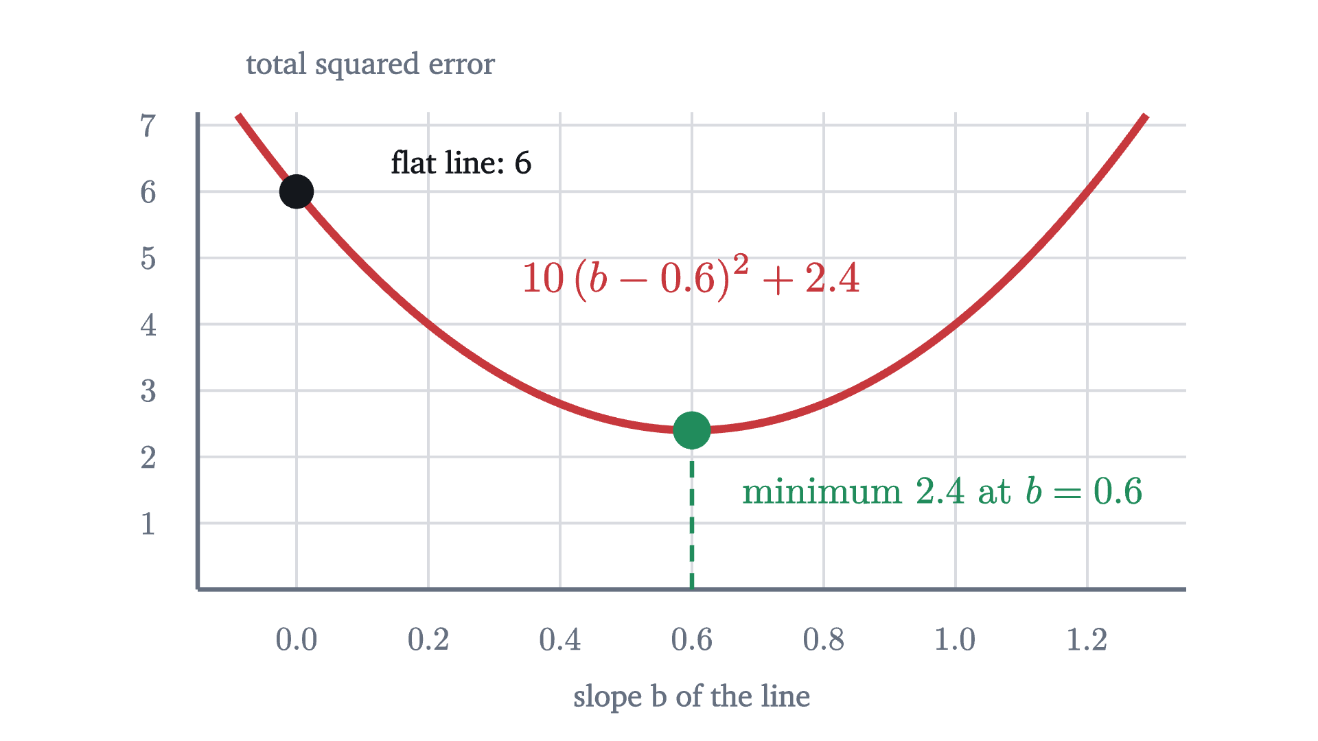
The animation suggests that the best line has slope 0.6 and passes through $(3, 4)$, the point whose coordinates are the mean of the $x$ values and the mean of the $y$ values. An animation tries only some lines. We want a proof that covers all of them, and a formula that works for any data.

Deriving the least-squares line

Let the data be $(x_1, y_1), \dots, (x_n, y_n)$, with means $\bar x$ and $\bar y$, and suppose the $x_i$ are not all equal. The quantity to minimize is

Q(a, b) = \sum_{i=1}^{n} \bigl(y_i - a - bx_i\bigr)^2.

The means are the natural reference point, so measure everything from them. Write $u_i = x_i - \bar x$ and $v_i = y_i - \bar y$ for the deviations, and note that $\sum u_i = 0$ and $\sum v_i = 0$, because deviations from a mean always sum to zero. Three sums will appear over and over:

S_{xx} = \sum u_i^2, \qquad S_{yy} = \sum v_i^2, \qquad S_{xy} = \sum u_i v_i.

For the five students, $u = (-2, -1, 0, 1, 2)$ and $v = (-2, 0, 1, 0, 1)$, so $S_{xx} = 10$, $S_{yy} = 6$ and $S_{xy} = 4 + 0 + 0 + 0 + 2 = 6$.

Proof

Substitute $x_i = \bar x + u_i$ and $y_i = \bar y + v_i$ into a residual:

y_i - a - bx_i = (v_i - bu_i) + c, \qquad \text{where } c = \bar y - a - b\bar x.

The number $c$ is the same for every $i$: it is the vertical gap between the point of means and the line. Squaring and summing,

Q = \sum (v_i - bu_i)^2 + 2c\sum (v_i - bu_i) + nc^2.

The middle sum is $\sum v_i - b\sum u_i = 0$. So

Q = \sum (v_i - bu_i)^2 + nc^2 = S_{yy} - 2bS_{xy} + b^2 S_{xx} + nc^2.

The first three terms form a quadratic in $b$ with leading coefficient $S_{xx}$, which is positive because the $x_i$ are not all equal. Complete the square:

S_{xx}b^2 - 2S_{xy}b + S_{yy} = S_{xx}\Bigl(b - \frac{S_{xy}}{S_{xx}}\Bigr)^2 + S_{yy} - \frac{S_{xy}^2}{S_{xx}}.

Therefore

Q(a, b) = S_{xx}\Bigl(b - \frac{S_{xy}}{S_{xx}}\Bigr)^2 + nc^2 + \Bigl(S_{yy} - \frac{S_{xy}^2}{S_{xx}}\Bigr).

The last bracket does not involve $a$ or $b$. The first two terms are squares with positive coefficients, so each is at least 0, and both are 0 exactly when $b = S_{xy}/S_{xx}$ and $c = 0$, that is, $a = \bar y - b\bar x$. At that one point $Q$ equals the last bracket, and everywhere else it is larger.

Each term has a meaning. The term $nc^2$ is the penalty for a line that misses the point of means, and it vanishes when $c = 0$: the best line always passes through $(\bar x, \bar y)$. The term with $b$ is the penalty for a wrong tilt. A reader who knows calculus can reach the same formulas by setting the derivatives of $Q$ with respect to $a$ and $b$ to zero, as in the lesson on optimization. Completing the square has the advantage of proving at the same stroke that the point found is a minimum and the only one.

For the five students, $b = 6/10 = 0.6$ and $a = 4 - 0.6 \times 3 = 2.2$. The best line is $y = 2.2 + 0.6x$, and its total squared error is $6 - 36/10 = 2.4$, as the animation found.

The total squared error of lines through the point of means (3, 4), as a function of their slope b, for the five students. It is the parabola 10(b - 0.6)^2 + 2.4, lowest at slope 0.6. A flat line, slope 0, has error S_{yy} = 6. — The total squared error of lines through the point of means $(3, 4)$, as a function of their slope $b$, for the five students. It is the parabola $10(b - 0.6)^2 + 2.4$, lowest at slope 0.6. A flat line, slope 0, has error $S_{yy} = 6$.

Correlation: how tightly the points follow the line

The slope tells us how steep the line is. It does not tell us how well the points stick to it, and it changes if we change units: measure practice in minutes and the slope becomes 0.01. We want a measure of the strength of the linear association that ignores units.

The sum $S_{xy} = \sum (x_i - \bar x)(y_i - \bar y)$ already detects association. A point above both means, or below both, contributes a positive product. A point above one mean and below the other contributes a negative product. If high $x$ tends to go with high $y$, positive products dominate.

The father-son data divided at the two means. In the blue quadrants both heights lie on the same side of their means, and the product of deviations is positive. In the orange quadrants they lie on opposite sides. Two thirds of the pairs are blue, which is what makes the correlation positive.

$S_{xy}$ still depends on the units and on $n$. Dividing by the geometric mean of $S_{xx}$ and $S_{yy}$ removes both.

The condition that neither variable is constant keeps the denominator from being zero. Since the sample standard deviations are $s_x = \sqrt{S_{xx}/(n-1)}$ and $s_y = \sqrt{S_{yy}/(n-1)}$, the same number can be written $r = \frac{1}{n-1}\sum \frac{x_i - \bar x}{s_x} \cdot \frac{y_i - \bar y}{s_y}$: the average product of the two variables once each is expressed in standard deviations from its mean. Changing units rescales a deviation and its standard deviation together, so $r$ has no units.

Pause and try

Compute $r$ for the five students, using $S_{xx} = 10$, $S_{yy} = 6$, $S_{xy} = 6$.

Show answerHide answer

$r = \dfrac{6}{\sqrt{10 \times 6}} = \dfrac{6}{\sqrt{60}} \approx 0.775$.

For the simulated fathers and sons, $r = 0.51$. How large can $r$ be? The answer comes from a famous inequality, and we already hold its proof.

What $r^2$ measures

The least-squares theorem gave the smallest possible total squared error as $S_{yy} - S_{xy}^2/S_{xx}$. Factor out $S_{yy}$ and the definition of $r$ appears:

\text{minimum of } Q = S_{yy}\Bigl(1 - \frac{S_{xy}^2}{S_{xx}S_{yy}}\Bigr) = S_{yy}\,(1 - r^2).

Now $S_{yy}$ is itself a total squared error: it is the error of the flat line $y = \bar y$, the best prediction available to someone who ignores $x$ altogether. So $1 - r^2$ is the fraction of that error which remains after the line is fitted, and $r^2$ is the fraction removed.

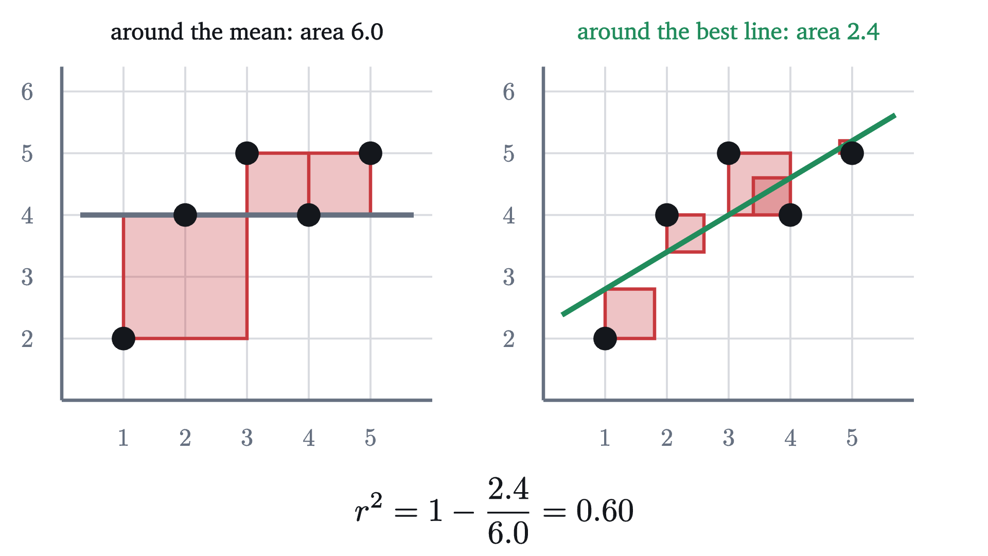
The same five points measured two ways. Left: squares on the deviations from the mean score, the flat line at 4, with total area S_{yy} = 6. Right: squares on the residuals from the least-squares line, with total area 2.4. The line removes 60% of the squared error, and r^2 = 0.6. — The same five points measured two ways. Left: squares on the deviations from the mean score, the flat line at 4, with total area $S_{yy} = 6$. Right: squares on the residuals from the least-squares line, with total area 2.4. The line removes 60% of the squared error, and $r^2 = 0.6$.

The fraction is sobering for moderate correlations. The fathers and sons have $r \approx 0.5$, so $r^2 \approx 0.25$: knowing the father’s height removes only a quarter of the squared error in predicting the son’s.

Regression to the mean

The slope and the correlation are connected. Because $b = \frac{S_{xy}}{S_{xx}}$ and $r = \frac{S_{xy}}{\sqrt{S_{xx}S_{yy}}}$,

b = r\,\sqrt{\frac{S_{yy}}{S_{xx}}} = r\,\frac{s_y}{s_x}.

Put this into the line $\hat y - \bar y = b(x - \bar x)$, where $\hat y$ denotes the predicted value, and divide by $s_y$:

\frac{\hat y - \bar y}{s_y} = r \cdot \frac{x - \bar x}{s_x}.

In words: if $x$ is $z$ standard deviations above its mean, the predicted $y$ is $rz$ standard deviations above its mean.

Pause and try

Take fathers and sons to have mean 176 cm and standard deviation 7 cm in both generations, with $r = 0.5$. A father is 190 cm tall. What does the regression line predict for his son? And if all you know is that a son is 190 cm, what is the prediction for his father?

Show answerHide answer

The father is $(190 - 176)/7 = 2$ standard deviations above the mean. The prediction for the son is $0.5 \times 2 = 1$ standard deviation above, which is 183 cm, not 190. The second question has the same answer by the same calculation with the roles exchanged: the predicted father of a 190 cm son is 183 cm, not 204.

Since $|r| < 1$ unless the data are perfectly linear, the prediction for any $x$ other than $\bar x$ is fewer standard deviations from the mean than the input. This is regression to the mean, and the second half of that answer shows that it has nothing to do with the passage of time. Tall sons have fathers who are, on average, shorter than they are.

The dashed line marks sons exactly as tall as their fathers. If height were simply copied, the cloud would lie along it.
Fathers between 182 and 186 cm average 183.9 cm. Their sons average 181.3 cm: tall, but closer to the mean than their fathers. The ring is below the dashed line.
Fathers between 166 and 170 cm average 168.1 cm, and their sons average 171.7 cm. The ring is above the dashed line.
Now select by the sons. Sons between 182 and 186 cm average 183.5 cm, and their fathers average only 180.3 cm. Regression runs both ways.

Regression to the mean in the father-son data, in both directions. Fathers in a tall band have sons who average less than the fathers do, and fathers in a short band have sons who average more. But sons in a tall band also have fathers who average less than the sons do.

Monocurl source

let Band = |use_f, lo, hi, col| {
    let key = [SONS, FATHERS][use_f]
    let sel = filter(range(0, NPAIR), |i| key[i] >= lo and key[i] < hi and inside(FATHERS[i], SONS[i]))
    let mf = mean(map(sel, |i| FATHERS[i]))
    let ms = mean(map(sel, |i| SONS[i]))
    var box = [at(ff, lo, 154), at(ff, hi, 154), at(ff, hi, 198), at(ff, lo, 198)]
    if (not use_f) {
        box = [at(ff, 154, lo), at(ff, 198, lo), at(ff, 198, hi), at(ff, 154, hi)]
    }
    return [
        Region(box, tint(col, 0.14)),
        map(sel, |i| Pt(at(ff, FATHERS[i], SONS[i]), col, 0.055)),
        Ring(at(ff, mf, ms), INK, 0.13, 4),
        [mf, ms]
    ]
}
# one row above the plot, clear of the grid: each piece starts where the last one ends
let Readout = |top, a, bottom, b, col| {
    let t1 = center{[-0.8, 1.93, 0]} Cap(top, 0.7, col)
    let n1 = next_to{t1, 1r, 0.12} Math(str_join([to_string(a, 1), "\text{ cm}"]), 0.8, col)
    let t2 = next_to{n1, 1r, 0.36} Cap(bottom, 0.7, col)
    let n2 = next_to{t2, 1r, 0.12} Math(str_join([to_string(b, 1), "\text{ cm}"]), 0.8, col)
    return [t1, n1, t2, n2]
}
let T = Band(1, 182, 186, EMBER)
let S = Band(1, 166, 170, PLUM)
let U = Band(0, 182, 186, GOLD)
mesh plot = [HeightPlot, SonName]
mesh cloud = map(filter(range(0, NPAIR), |i| inside(FATHERS[i], SONS[i])), |i| Pt(at(ff, FATHERS[i], SONS[i]), alpha{0.45} AZURE, 0.04))
mesh same = SameLine
mesh band = []
mesh note = []

slide "The dashed line marks sons exactly as tall as their fathers. If height were simply copied, the cloud would lie along it."
    play Fade(0.6)

slide "Fathers between 182 and 186 cm average 183.9 cm. Their sons average 181.3 cm: tall, but closer to the mean than their fathers. The ring is below the dashed line."
    band = take(T, 3)
    note = Readout("these fathers:", T[3][0], "their sons:", T[3][1], EMBER)
    play Fade(0.7, [&band, &note])

slide "Fathers between 166 and 170 cm average 168.1 cm, and their sons average 171.7 cm. The ring is above the dashed line."
    band = []
    note = []
    play Fade(0.4, [&band, &note])
    band = take(S, 3)
    note = Readout("these fathers:", S[3][0], "their sons:", S[3][1], PLUM)
    play Fade(0.7, [&band, &note])

slide "Now select by the sons. Sons between 182 and 186 cm average 183.5 cm, and their fathers average only 180.3 cm. Regression runs both ways."
    band = []
    note = []
    play Fade(0.4, [&band, &note])
    band = take(U, 3)
    note = Readout("these sons:", U[3][1], "their fathers:", U[3][0], INK)
    play Fade(0.7, [&band, &note])

Uses the shared definitions for this lesson's figures.

Here is the resolution of the opening paradox. A father’s height only partly determines his son’s. Among fathers of 190 cm, the sons scatter around 183 cm, with a spread nearly as large as that of the whole population: the leftover fraction is $1 - r^2 = 0.75$ of the variance. Some of those sons are 195 cm. Meanwhile, some sons of average fathers are 190 cm too. The very tall men of the next generation are supplied by fathers of every height, mostly ones shorter than themselves. The averages regress, the scatter restores the spread, and the distribution of heights stays the same from one generation to the next.

Regression to the mean appears wherever two measurements are imperfectly correlated. Students with the highest scores on a first test score lower, on average, on the second, and those with the lowest scores improve. No explanation in terms of effort or complacency is needed, although one is nearly always offered.

Correlation is not causation

A correlation says that two variables move together in the data. It does not say why. Over a year of days in a seaside town, ice cream sales and the number of swimmers rescued by lifeguards are strongly correlated. Nobody concludes that ice cream makes people drown.

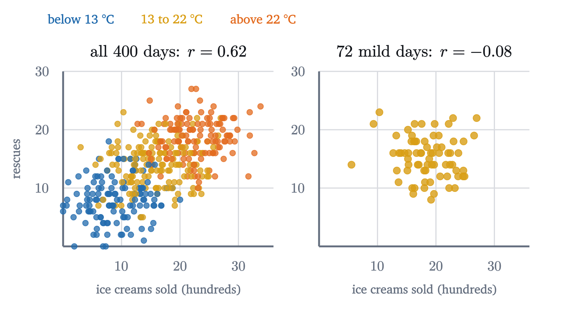
A simulation of 400 days in a seaside town. Each day's temperature raises both ice cream sales and lifeguard rescues, and neither affects the other. Left: across all days the two are clearly correlated. Right: among days with nearly the same temperature, 18 to 22 °C, the correlation is gone. — A simulation of 400 days in a seaside town. Each day’s temperature raises both ice cream sales and lifeguard rescues, and neither affects the other. Left: across all days the two are clearly correlated. Right: among days with nearly the same temperature, 18 to 22 °C, the correlation is gone.

In the simulation $r = 0.62$ across all 400 days. Hot days are in the upper right of the cloud and cold days in the lower left, and that arrangement is the whole correlation. Among the 72 days when the temperature was between 18 and 22 °C, $r = -0.08$, which is indistinguishable from zero. Temperature here is a confounder, or lurking variable: a third quantity that influences both of the others. Holding it nearly fixed removes the association it created.

When $x$ and $y$ are correlated, at least four explanations are open: $x$ influences $y$; $y$ influences $x$; a third variable influences both; or the correlation is a chance pattern in a small sample, which is a question for a hypothesis test. The data alone cannot choose among them. What can is an experiment in which the experimenter sets $x$ by a random device, so that nothing else can be systematically tied to it. Give out free ice cream on randomly chosen days, and the rescues will not change.

Worked examples

What $r$ does not see

The correlation coefficient measures how well a straight line describes the data, and nothing else. In 1973 the statistician Francis Anscombe published four small data sets to make the point.

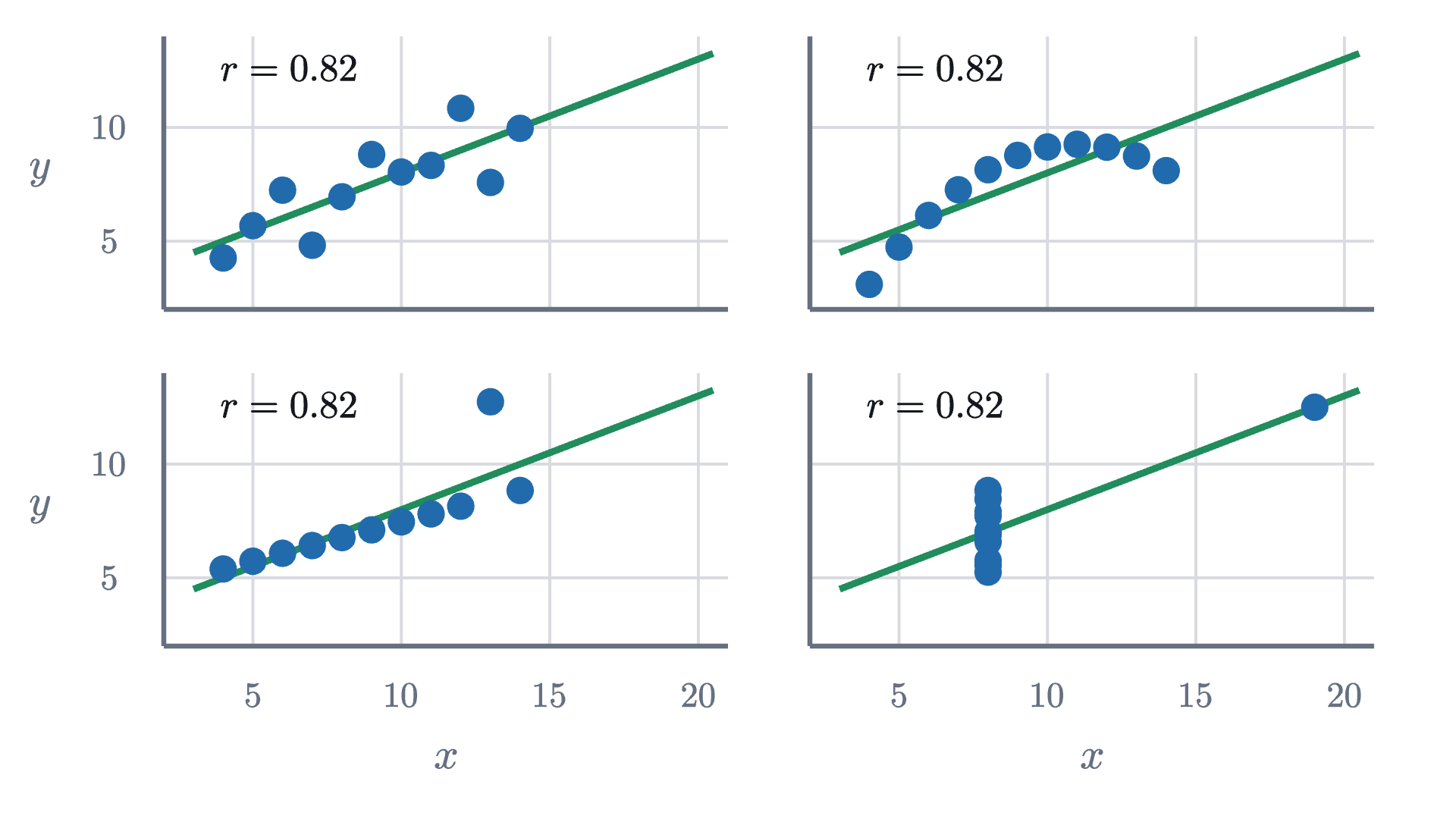
Anscombe's four data sets, each with 11 points. All four have the same means, the same least-squares line y = 3 + 0.5x (green) and the same correlation, 0.82. Only the first is the kind of cloud those numbers suggest. The others are a curve, a line with one outlier, and a vertical stack with one far point that creates the whole correlation. — Anscombe’s four data sets, each with 11 points. All four have the same means, the same least-squares line $y = 3 + 0.5x$ (green) and the same correlation, 0.82. Only the first is the kind of cloud those numbers suggest. The others are a curve, a line with one outlier, and a vertical stack with one far point that creates the whole correlation.

A strong relationship can also have no correlation at all. For the five points $(-2, 4), (-1, 1), (0, 0), (1, 1), (2, 4)$, which lie exactly on the curve $y = x^2$, we get $\bar x = 0$ and $S_{xy} = \sum x_i(y_i - \bar y) = -8 - 1 + 0 + 1 + 8 - \bar y \sum x_i = 0$, so $r = 0$. Here $y$ is completely determined by $x$, and $r$ reports nothing, because the relationship is not linear. Always look at the scatter plot before trusting $r$.

Stepping back

The hard step was the first one: deciding what “best line” should mean, and then showing that the choice has a single answer with a formula. Completing the square did that, and the same line of algebra then handed us the bound on $r$ and the meaning of $r^2$ at no extra cost. One identity, $Q = S_{xx}(b - S_{xy}/S_{xx})^2 + nc^2 + S_{yy}(1 - r^2)$, contains the slope, the intercept, the Cauchy-Schwarz inequality and the fraction of variation explained.

The limits matter as much as the formulas. The line describes averages, and individuals scatter around it. The correlation sees only straight-line patterns. And neither says anything about cause until someone runs an experiment.

Check yourself

In a large group of adults, height and weight have correlation $r = 0.7$. Which conclusion is justified?

Recap

The least-squares line minimizes the sum of squared vertical misses. It has slope $b = S_{xy}/S_{xx}$ and passes through the point of means: $a = \bar y - b\bar x$.
The proof completes the square: $Q(a, b) = S_{xx}(b - S_{xy}/S_{xx})^2 + nc^2 + S_{yy} - S_{xy}^2/S_{xx}$, with $c = \bar y - a - b\bar x$.
The correlation is $r = S_{xy}/\sqrt{S_{xx}S_{yy}}$. By the Cauchy-Schwarz inequality $-1 \le r \le 1$, with $\pm 1$ only for points on a line.
The minimum squared error is $S_{yy}(1 - r^2)$, so $r^2$ is the fraction of the variation in $y$ accounted for by the line.
In standard units the line is $\hat z_y = r z_x$. Since $|r| < 1$, predictions are closer to the mean than the inputs: regression to the mean, in both directions.
Correlation can come from a confounder, and $r$ misses curved relationships and is swayed by outliers. Plot the data.

Problems

The first three are computations. The next four ask for reasons. The last is a challenge.

Problem 1

Find the least-squares line, $r$ and $r^2$ for the points $(1, 2), (2, 3), (3, 5), (4, 6)$.

Show solutionHide solution

$\bar x = 2.5$ and $\bar y = 4$. Deviations: $u = (-1.5, -0.5, 0.5, 1.5)$, $v = (-2, -1, 1, 2)$. $S_{xx} = 2.25 + 0.25 + 0.25 + 2.25 = 5$, $S_{yy} = 4 + 1 + 1 + 4 = 10$, $S_{xy} = 3 + 0.5 + 0.5 + 3 = 7$. Slope $b = 7/5 = 1.4$, intercept $a = 4 - 1.4 \times 2.5 = 0.5$, so the line is $y = 0.5 + 1.4x$. $r = 7/\sqrt{50} \approx 0.990$ and $r^2 = 49/50 = 0.98$.

Problem 2

For a set of data, $\bar x = 50$, $s_x = 10$, $\bar y = 70$, $s_y = 8$ and $r = 0.6$. Find the regression line of $y$ on $x$ and the predicted $y$ at $x = 65$.

Show solutionHide solution

$b = r s_y/s_x = 0.6 \times 8/10 = 0.48$, and $a = \bar y - b\bar x = 70 - 24 = 46$. The line is $\hat y = 46 + 0.48x$. At $x = 65$: $\hat y = 46 + 31.2 = 77.2$. Check in standard units: $x$ is 1.5 standard deviations above its mean, so $\hat y$ is $0.9$ above, $70 + 0.9 \times 8 = 77.2$.

Problem 3

Two variables have $r = -0.9$. (a) What fraction of the squared variation in $y$ does the regression line account for? (b) If $x$ is 1 standard deviation above its mean, what is the prediction for $y$? (c) Is the association weaker than one with $r = 0.5$?

Show solutionHide solution

(a) $r^2 = 0.81$. (b) $-0.9$ standard deviations: below the mean of $y$ by nine tenths of a standard deviation. (c) No, it is much stronger. The sign of $r$ gives the direction of the line and $|r|$ gives the strength; $r = 0.5$ accounts for only 25% of the variation.

Problem 4

Show that the residuals of the least-squares line always sum to zero. Is the same true of any line through the point of means?

Show solutionHide solution

The residuals are $y_i - a - bx_i$. Their sum is $\sum y_i - na - b\sum x_i = n\bar y - na - bn\bar x = n(\bar y - a - b\bar x)$. For the least-squares line $a = \bar y - b\bar x$, so this is zero. The calculation used only that relation between $a$ and $b$, and not the value of $b$. A line passes through $(\bar x, \bar y)$ exactly when $\bar y = a + b\bar x$, so yes: the residuals sum to zero for every line through the point of means, and for no other line.

Problem 5

Heights $x$ are recorded in centimeters and weights $y$ in kilograms, giving slope $b$, intercept $a$ and correlation $r$. The heights are then converted to meters, $x' = x/100$. Find the new slope, intercept and correlation.

Show solutionHide solution

The new deviations are $u_i' = u_i/100$, so $S_{x'x'} = S_{xx}/10^4$ and $S_{x'y} = S_{xy}/100$, while $S_{yy}$ is unchanged. The new slope is $\frac{S_{xy}/100}{S_{xx}/10^4} = 100b$ (kilograms per meter is 100 times kilograms per centimeter). The new intercept is $\bar y - 100b \cdot \bar x/100 = a$, unchanged. The new correlation is $\frac{S_{xy}/100}{\sqrt{S_{xx}S_{yy}}/100} = r$, unchanged.

Problem 6

Besides the regression line of $y$ on $x$, one can fit the regression line of $x$ on $y$, which predicts $x$ from $y$ and minimizes squared horizontal misses; by symmetry its equation is $x - \bar x = b'(y - \bar y)$ with $b' = S_{xy}/S_{yy}$. (a) Show that $bb' = r^2$. (b) Drawn on the same axes, with $x$ horizontal, what are the slopes of the two lines when both variables have the same standard deviation and $r = 0.5$? (c) When do the two lines coincide?

Show solutionHide solution

(a) $bb' = \frac{S_{xy}}{S_{xx}} \cdot \frac{S_{xy}}{S_{yy}} = \frac{S_{xy}^2}{S_{xx}S_{yy}} = r^2$. (b) With equal standard deviations, $b = b' = r = 0.5$. The first line has slope 0.5. The second is $x - \bar x = 0.5(y - \bar y)$, which in the usual orientation is $y - \bar y = 2(x - \bar x)$, slope 2. Both pass through the point of means, one flatter than the diagonal and one steeper. This is regression to the mean in both directions. (c) If $r = 0$ the lines are horizontal and vertical. Otherwise the second line has slope $1/b'$ in the usual orientation, so they coincide when $b = 1/b'$, that is, $bb' = r^2 = 1$: only when the points lie exactly on a line.

Problem 7

Compute $r$ for the four points $(-1, 1), (0, 0), (1, 1), (2, 4)$ on the curve $y = x^2$, and compare with the lesson’s example where $r = 0$. What made the difference?

Show solutionHide solution

$\bar x = 0.5$, $\bar y = 1.5$. Deviations: $u = (-1.5, -0.5, 0.5, 1.5)$, $v = (-0.5, -1.5, -0.5, 2.5)$. $S_{xx} = 5$, $S_{yy} = 0.25 + 2.25 + 0.25 + 6.25 = 9$, $S_{xy} = 0.75 + 0.75 - 0.25 + 3.75 = 5$. So $r = 5/\sqrt{45} \approx 0.745$. The curve is the same, but these $x$ values are not symmetric about 0: most of them are on the rising side of the parabola, where a line is a fair description. The value of $r$ depends on which part of a curved relationship was sampled, another reason to look at the plot.

Problem 8

(An association that reverses.) Six measurements fall in two groups. Group A: $(1, 3), (2, 2), (3, 1)$. Group B: $(6, 8), (7, 7), (8, 6)$. (a) Find $r$ within each group. (b) Find $r$ for all six points together. (c) Explain how both can be true, and what it means for interpreting a correlation.

Show solutionHide solution

(a) In group A the points satisfy $y = 4 - x$ exactly, and in group B they satisfy $y = 14 - x$. Points on a line of negative slope have $r = -1$ in each group.

(b) For all six, $\bar x = 27/6 = 4.5$ and $\bar y = 27/6 = 4.5$. Deviations: $u = (-3.5, -2.5, -1.5, 1.5, 2.5, 3.5)$ and $v = (-1.5, -2.5, -3.5, 3.5, 2.5, 1.5)$. $S_{xx} = 2(12.25 + 6.25 + 2.25) = 41.5$, and $S_{yy} = 41.5$ likewise. $S_{xy} = 5.25 + 6.25 + 5.25 + 5.25 + 6.25 + 5.25 = 33.5$. So $r = 33.5/41.5 \approx 0.81$.

(c) Within each group, larger $x$ goes with smaller $y$. But group B sits higher than group A on both variables, and the difference between the groups dominates the pooled data. The group label is a confounder: it influences both $x$ and $y$. Pooled, the correlation is strongly positive; holding the group fixed, it is perfectly negative. A correlation computed across a mixed population can differ in size, and even in sign, from the relationship inside every subgroup, so a correlation alone cannot tell you what would happen to $y$ if you changed $x$.

Shared definitions used by this lesson's figures

# house kit: prepended to every essay figure after the std imports

# palette. AZURE and EMBER are the two actors, LEAF marks an answer, ROSE a problem
let PAPER = [1, 1, 1, 1]
let INK = [0.08, 0.09, 0.11, 1]
let SLATE = [0.40, 0.44, 0.50, 1]
let MIST = [0.85, 0.86, 0.88, 1]
let AZURE = [0.13, 0.42, 0.68, 1]
let EMBER = [0.89, 0.42, 0.12, 1]
let LEAF = [0.13, 0.55, 0.36, 1]
let ROSE = [0.78, 0.22, 0.24, 1]
let PLUM = [0.47, 0.30, 0.66, 1]
let GOLD = [0.85, 0.62, 0.08, 1]

background = PAPER

# an opaque pastel of col; use for fills so overlaps do not darken
let tint = |col, amount = 0.18| [
    1 - (1 - col[0]) * amount,
    1 - (1 - col[1]) * amount,
    1 - (1 - col[2]) * amount,
    1
]

# text: Cap for labels, Note for quiet labels, Math for typeset maths
let Cap = |txt, size = 0.75, col = INK| color{col} Text(txt, size, "Charter")
let Note = |txt, size = 0.65| color{SLATE} Text(txt, size, "Charter")
let Math = |tex, size = 0.9, col = INK| color{col} Tex(tex, size)

# a paper rectangle to sit behind text that crosses lines
let Plate = |pos, size| center{pos} fill{PAPER} stroke{alpha{0} PAPER, 0} Rect(size)

# shapes with fill and stroke both set, so no stray black appears
let Pt = |pos, col = INK, r = 0.075| center{pos} fill{col} stroke{col, 1} Circle(r, 48)
let Ring = |pos, col = INK, r = 0.1, w = 3| center{pos} fill{PAPER} stroke{col, w} Circle(r, 48)
let Seg = |a, b, col = INK, w = 3| stroke{col, w} Line(a, b)
let Path = |pts, col = INK, w = 3| stroke{col, w} Polyline(pts)
let Region = |pts, col| fill{col} stroke{alpha{0} col, 0} Polygon(pts)
let Outline = |pts, col = INK, w = 3| fill{alpha{0} PAPER} stroke{col, w} Polygon(pts)
let Shape = |pts, col, amount = 0.18, w = 3| fill{tint(col, amount)} stroke{col, w} Polygon(pts)
let Disc = |pos, r, col, amount = 0.18, w = 3| center{pos} fill{tint(col, amount)} stroke{col, w} Circle(r, 96)
let Box = |pos, size, col, amount = 0.18, w = 3| center{pos} fill{tint(col, amount)} stroke{col, w} Rect(size)
# a line from a to b ending in a small solid arrowhead
let Tip = |a, b, col = INK, w = 3, head = 0.17| {
    let d = normalize([b[0] - a[0], b[1] - a[1], 0])
    let n = [-d[1], d[0], 0]
    let base = [b[0] - d[0] * head, b[1] - d[1] * head, 0]
    return [
        stroke{col, w} Line(a, base),
        fill{col} stroke{col, 1} Polygon([
            b,
            [base[0] + n[0] * head * 0.42, base[1] + n[1] * head * 0.42, 0],
            [base[0] - n[0] * head * 0.42, base[1] - n[1] * head * 0.42, 0]
        ])
    ]
}

# plots. a frame is [x0, x1, y0, y1, centre, width, height]: a data window and the scene box it fills
let Frame = |x0, x1, y0, y1, c = [0, 0, 0], w = 6.4, h = 3.6| [x0, x1, y0, y1, c, w, h]
let fx = |fr, x| fr[4][0] + (x - (fr[0] + fr[1]) / 2) * fr[5] / (fr[1] - fr[0])
let fy = |fr, y| fr[4][1] + (y - (fr[2] + fr[3]) / 2) * fr[6] / (fr[3] - fr[2])
let at = |fr, x, y| [fx(fr, x), fy(fr, y), 0]

# axes through the data origin (or the nearest edge of the window), with optional names
let Axes = |fr, x_name = "", y_name = "", col = SLATE| {
    let ox = clamp(fr[0], 0, fr[1])
    let oy = clamp(fr[2], 0, fr[3])
    var parts = [
        Tip(at(fr, fr[0], oy), [fx(fr, fr[1]) + 0.25, fy(fr, oy), 0], col, 2.5, 0.15),
        Tip(at(fr, ox, fr[2]), [fx(fr, ox), fy(fr, fr[3]) + 0.25, 0], col, 2.5, 0.15)
    ]
    if (x_name != "") {
        parts .= center{[fx(fr, fr[1]) + 0.5, fy(fr, oy), 0]} Math(x_name, 0.8, col)
    }
    if (y_name != "") {
        parts .= center{[fx(fr, ox), fy(fr, fr[3]) + 0.5, 0]} Math(y_name, 0.8, col)
    }
    return parts
}

# tick marks with numbers at the listed data values
let XTicks = |fr, xs, col = SLATE, places = 0| block {
    let oy = fy(fr, clamp(fr[2], 0, fr[3]))
    for (x in xs) {
        . Seg([fx(fr, x), oy - 0.07, 0], [fx(fr, x), oy + 0.07, 0], col, 2)
        . center{[fx(fr, x), oy - 0.33, 0]} Math(to_string(x, places), 0.72, col)
    }
}
let YTicks = |fr, ys, col = SLATE, places = 0| block {
    let ox = fx(fr, clamp(fr[0], 0, fr[1]))
    for (y in ys) {
        . Seg([ox - 0.07, fy(fr, y), 0], [ox + 0.07, fy(fr, y), 0], col, 2)
        . center{[ox - 0.36, fy(fr, y), 0]} Math(to_string(y, places), 0.72, col)
    }
}

# faint grid lines at the listed data values
let GridLines = |fr, xs, ys, col = MIST| block {
    for (x in xs) {
        . Seg(at(fr, x, fr[2]), at(fr, x, fr[3]), col, 1.5)
    }
    for (y in ys) {
        . Seg(at(fr, fr[0], y), at(fr, fr[1], y), col, 1.5)
    }
}

# the graph of f over [a, b], drawn in the frame. values are clamped to the window
let Graph = |fr, f, a, b, col = AZURE, w = 4, n = 160|
    stroke{col, w} Polyline(map(sample(a, b, n), |x| at(fr, x, clamp(fr[2], f(x), fr[3]))))

# the region between the graph of f and the x axis over [a, b]
let AreaUnder = |fr, f, a, b, col = AZURE, amount = 0.2, n = 80| {
    var pts = [at(fr, a, 0)]
    for (x in sample(a, b, n)) {
        pts .= at(fr, x, clamp(fr[2], f(x), fr[3]))
    }
    pts .= at(fr, b, 0)
    return fill{tint(col, amount)} stroke{alpha{0} col, 0} Polygon(pts)
}

let rnd = |i, salt| mod(seeded_random(i, salt) + 1, 1)
let std_normal = |i, salt| sqrt(-2 * ln(max(rnd(i, salt), 0.000000001))) * cos(TAU * rnd(i, salt + 1))
# sums of products of deviations, correlation, least-squares slope and intercept
let sxy = |xs, ys| {
    let mx = mean(xs)
    let my = mean(ys)
    return sum(map(range(0, len(xs)), |i| (xs[i] - mx) * (ys[i] - my)))
}
let corr = |xs, ys| sxy(xs, ys) / sqrt(sxy(xs, xs) * sxy(ys, ys))
let slope = |xs, ys| sxy(xs, ys) / sxy(xs, xs)
let icept = |xs, ys| mean(ys) - slope(xs, ys) * mean(xs)
# simulated heights of 300 fathers and their adult sons: mean 176 cm, sd 7 cm, correlation 0.5
let NPAIR = 300
let FATHERS = map(range(0, NPAIR), |i| 176 + 7 * std_normal(i + 1, 61))
let SONS = map(range(0, NPAIR), |i| 176 + 0.5 * (FATHERS[i] - 176) + 7 * sqrt(0.75) * std_normal(i + 1, 63))
let FB = slope(FATHERS, SONS)
let FA = icept(FATHERS, SONS)
let ff = Frame(154, 198, 154, 198, [0.25, 0.1, 0], 5.9, 3.0)
let HeightPlot = [
    GridLines(ff, [160, 170, 180, 190], [160, 170, 180, 190]),
    Seg(at(ff, 154, 154), at(ff, 198, 154), SLATE, 2.5),
    Seg(at(ff, 154, 154), at(ff, 154, 198), SLATE, 2.5),
    map([160, 170, 180, 190], |v| [
        center{[fx(ff, v), fy(ff, 154) - 0.3, 0]} Math(to_string(v), 0.72, SLATE),
        center{[fx(ff, 154) - 0.4, fy(ff, v), 0]} Math(to_string(v), 0.72, SLATE)
    ]),
    center{[fx(ff, 176), fy(ff, 154) - 0.66, 0]} Note("father's height (cm)", 0.74)
]
let SonName = center{[fx(ff, 154) + 0.25, fy(ff, 198) + 0.3, 0]} Note("son's height (cm)", 0.74)
let inside = |x, y| x > 154.5 and x < 197.5 and y > 154.5 and y < 197.5
let SameLine = stroke{SLATE, 3} dashed{[0.14, 0.09]} Line(at(ff, 155, 155), at(ff, 197, 197))
let FitLine = Seg(at(ff, 155, FA + FB * 155), at(ff, 197, FA + FB * 197), LEAF, 4.5)
# the small example: hours of practice and score for five students
let PX = [1, 2, 3, 4, 5]
let PY = [2, 4, 5, 4, 5]
let fp = Frame(0, 6, 1, 6.4, [-1.75, 0.12, 0], 3.3, 2.97)
let PointPlot = |fr| [
    GridLines(fr, [1, 2, 3, 4, 5], [2, 3, 4, 5, 6]),
    Seg(at(fr, 0, 1), at(fr, 6, 1), SLATE, 2.5),
    Seg(at(fr, 0, 1), at(fr, 0, 6.4), SLATE, 2.5),
    map([1, 2, 3, 4, 5], |v| center{[fx(fr, v), fy(fr, 1) - 0.3, 0]} Math(to_string(v), 0.72, SLATE)),
    map([2, 3, 4, 5, 6], |v| center{[fx(fr, 0) - 0.28, fy(fr, v), 0]} Math(to_string(v), 0.72, SLATE))
]
let PointNames = |fr| [
    center{[fx(fr, 3), fy(fr, 1) - 0.66, 0]} Note("hours of practice, x", 0.74),
    center{[fx(fr, 0) + 0.45, fy(fr, 6.4) + 0.28, 0]} Note("score, y", 0.74)
]
let Dots = |fr| map(range(0, 5), |i| Pt(at(fr, PX[i], PY[i]), INK, 0.09))
let LineOn = |fr, a, b, col| Seg(at(fr, 0.3, a + 0.3 * b), at(fr, 5.7, a + 5.7 * b), col, 4)
# a square on each vertical miss between the point and the line y = a + b x
let Squares = |fr, a, b| block {
    for (i in range(0, 5)) {
        let x = PX[i]
        let yh = a + b * x
        let e = abs(PY[i] - yh)
        let x2 = x + [e, -e][x > 3]
        if (e > 0.03) {
            . fill{alpha{0.3} ROSE} stroke{ROSE, 2.5} Polygon([at(fr, x, yh), at(fr, x2, yh), at(fr, x2, PY[i]), at(fr, x, PY[i])])
        }
    }
}
let sq_total = |a, b| sum(map(range(0, 5), |i| (PY[i] - a - b * PX[i]) ^ 2))