Random Walks Become Bells

Flip a fair coin. Move one step right for heads and one step left for tails. After one flip, there are only two possible positions. After two flips, there are three. After a hundred flips, the possible positions form a wide mound.

That mound is not an accident. It is the beginning of the central limit theorem. Repeated independent noise tends to look Gaussian.

The familiar bell curve is

\frac{1}{\sqrt{2\pi\sigma^2}}e^{-x^2/(2\sigma^2)}.

But before thinking about formulas, it is better to watch the shape form.

Loading runtime...

0.00s

live slideshowessay-2026-random-walks-become-bells-1.mcs

param steps = 4

background = BLACK
camera = Camera(4b)

let bell = |x, steps| exp(-x * x / (0.18 * steps + 0.5))

let BellCurve = |steps| block {
    . stroke{BLUE, 3} ExplicitFunc(|x| -1.1 + 1.9 * bell(x, steps), [-3, 3, 240])
}

let Diagram = |steps| block {
    . stroke{GRAY, 1} Line(start: [-3.2, -1.1, 0], end: [3.2, -1.1, 0])
    . BellCurve(steps)
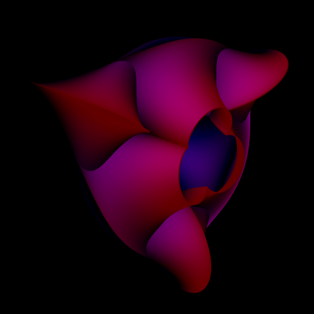
    . color{WHITE} center{[0, 1.45, 0]} Text("many small steps make a bell", 0.88)
}

mesh diagram = Diagram($steps)

slide "many steps"
    steps = 34
    play Lerp(1.6)

The image above does not show the exact binomial bars. It shows the limiting shape those bars approach after rescaling. The point is that the random walk does two things at once: it spreads out and it smooths out.

Probability shapes convolve

If $X$ and $Y$ are independent random variables, the distribution of $X+Y$ is a convolution of their distributions.

For discrete probabilities, convolution says:

P(X+Y=k)=\sum_j P(X=j)P(Y=k-j).

That sum is bookkeeping. To land at $k$, the first variable can land at $j$ while the second lands at $k-j$, and you add over all possible $j$.

For the coin walk, each new step convolves the current distribution with the tiny distribution

\frac12\delta_{-1}+\frac12\delta_1.

Each convolution spreads the mass a little and averages neighboring possibilities. This is why probability begins to look smooth even though the individual steps are discrete.

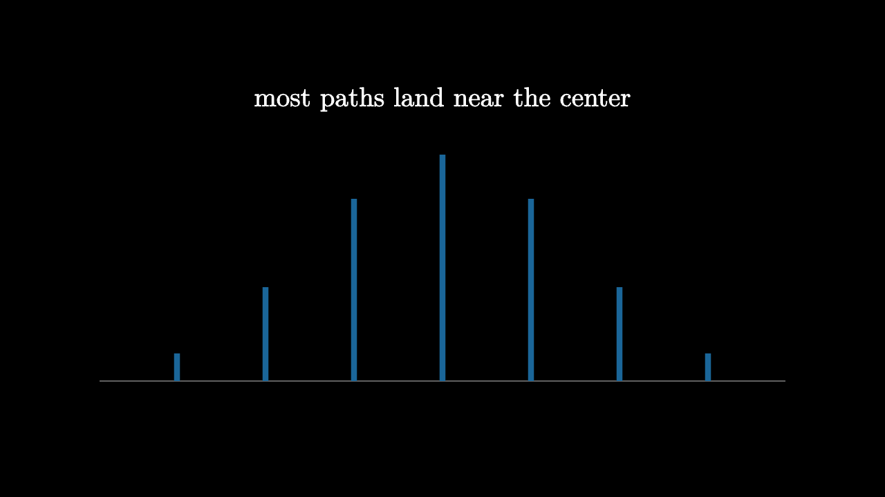
The binomial mound

After $n$ coin flips, the probability of getting $k$ heads is

\binom{n}{k}2^{-n}.

The position is $2k-n$. The coefficients in Pascal's triangle are therefore a random walk in disguise.

Near the center, these coefficients are large because there are many ways to get a balanced mixture of heads and tails. Far from the center, they are tiny because there are few ways to get mostly heads or mostly tails.

Why the Gaussian is special

The Gaussian is stable under convolution. Add two independent Gaussian variables and the result is another Gaussian. The variances add:

\sigma_{X+Y}^2=\sigma_X^2+\sigma_Y^2.

That stability is the reason the Gaussian appears as a fixed shape under repeated addition. Each new random contribution convolves the distribution with another small shape. After enough additions, the details of the original step distribution matter less than its mean and variance.

Fourier analysis gives the cleanest explanation. Convolution in position space becomes multiplication in frequency space. Repeated convolution raises a characteristic function to a high power. Near frequency zero, every reasonable distribution begins with the same quadratic behavior determined by variance. Raising that approximation to a high power produces the exponential quadratic shape of the Gaussian.

That paragraph is the central limit theorem in miniature.

What universality means

The central limit theorem is often paraphrased as "everything becomes normal." That is too loose. Heavy-tailed distributions can break the usual hypotheses. Dependence can change the limit. Scaling matters.

But under broad conditions, sums of many small independent contributions forget most details of the individual contributions. The limit remembers only the average drift and the variance.

That is universality. The bell curve is not common because nature loves one particular formula. It is common because many different microscopic stories lead to the same macroscopic shape when addition and independence dominate.

Random walks become bells because convolution keeps smoothing, spreading, and forgetting.