Bayes Tilts Belief

Bayes' rule is usually written as

The notation is compact, but it can make the idea feel like a symbolic trick. A better first picture is this: you begin with a distribution of belief over hypotheses. Then evidence arrives. Hypotheses that predicted the evidence get more weight. Hypotheses that made the evidence unlikely lose weight. Finally, the whole shape is rescaled so its total area is one again.

Bayesian updating is multiplication followed by normalization.

param evidence = 0.45

background = BLACK
camera = Camera(4b)

let prior = |x| exp(-0.75 * x * x)
let likelihood = |x, evidence| exp(-3.0 * (x - evidence) * (x - evidence))
let posterior = |x, evidence| prior(x) * likelihood(x, evidence) * 1.65

let PriorCurve = || block {
    . ExplicitFunc(|x| -1.15 + prior(x), [-3, 3, 240])
}

let LikelihoodCurve = |evidence| block {
    . ExplicitFunc(|x| -1.15 + likelihood(x, evidence), [-3, 3, 240])
}

let PosteriorCurve = |evidence| block {
    . ExplicitFunc(|x| -1.15 + posterior(x, evidence), [-3, 3, 240])
}

let Diagram = |evidence| block {
    . stroke{GRAY, 1} Line(start: [-3.2, -1.15, 0], end: [3.2, -1.15, 0])
    . stroke{ORANGE, 2} PriorCurve()
    . stroke{GREEN, 2} LikelihoodCurve(evidence)
    . stroke{BLUE, 3} PosteriorCurve(evidence)
    . color{WHITE} center{[0, 1.55, 0]} Text("posterior = prior x likelihood", 0.88)
}

mesh diagram = Diagram($evidence)

slide "move the evidence"
    evidence = -0.75
    play Lerp(1.4)

The orange curve is the prior. The green curve is the likelihood as a function of the hypothesis. The blue curve is proportional to their product. If evidence lands where the prior already had mass, the posterior becomes concentrated there. If evidence lands in a surprising place, the posterior compromises between prior expectation and the new observation.

The denominator is not the point

The denominator $P(E)$ is often the most intimidating part:

or in continuous form,

But geometrically, it is just the total mass after reweighting. Multiplying prior by likelihood changes the area under the curve. Dividing by $P(E)$ restores the area to $1$.

The update rule is therefore

That proportional sign is the conceptual heart of Bayes.

Evidence is not symmetric

The most common mistake is to confuse $P(E\mid H)$ with $P(H\mid E)$. If a disease almost always causes a positive test, that does not mean a positive test almost always implies the disease. The base rate matters.

Suppose a condition is rare. Even a good test may produce more false positives than true positives if it is applied to a large healthy population. Bayes' rule forces the prior probability into the calculation.

This is not philosophical caution. It is arithmetic. Evidence tilts belief, but it tilts the shape you already had. If the prior mass is tiny, a likelihood boost may still leave the posterior modest.

Log odds turn updates into addition

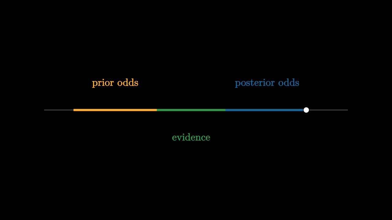
For two competing hypotheses, Bayesian updating has an elegant form in odds. The posterior odds equal prior odds times the likelihood ratio:

Taking logs turns this into addition:

Each piece of evidence adds a signed amount to the balance. Strong evidence is a large push. Weak evidence is a small nudge. Contradictory evidence pushes the other way.

imageessay-2026-bayes-tilts-belief-2.mcs

Copy

background = BLACK
camera = Camera(4b)

mesh diagram = block {
    . stroke{GRAY, 1} Line(start: [-3.1, 0, 0], end: [3.1, 0, 0])
    . stroke{ORANGE, 4} Line(start: [-2.5, 0, 0], end: [-0.8, 0, 0])
    . stroke{GREEN, 4} Line(start: [-0.8, 0, 0], end: [0.6, 0, 0])
    . stroke{BLUE, 4} Line(start: [0.6, 0, 0], end: [2.25, 0, 0])
    . fill{WHITE} center{[2.25, 0, 0]} Circle(0.06)
    . color{ORANGE} center{[-1.65, 0.55, 0]} Text("prior odds", 0.76)
    . color{GREEN} center{[-0.1, -0.55, 0]} Text("evidence", 0.76)
    . color{BLUE} center{[1.45, 0.55, 0]} Text("posterior odds", 0.76)
}

slide "log odds add"
    play Fade(0.6)

The shape of learning

Bayesian reasoning is not about blindly trusting priors, and it is not about blindly trusting data. It is about having a rule for how evidence changes a state of uncertainty.

A strong prior can resist weak evidence. Repeated evidence can overwhelm a strong prior. Precise measurements make narrow likelihoods. Noisy measurements make broad likelihoods. All of these cases are the same geometric operation: multiply the prior shape by the likelihood shape and renormalize.

Bayes' rule becomes much less mysterious when you stop treating it as a fraction and start treating it as a motion of probability mass.