The Laplace Transform Turns Memory Into Algebra

The Fourier transform asks what frequencies live inside a signal. The Laplace transform asks a related but broader question: how much of the signal remains after you discount the future exponentially?

For a function $f(t)$ defined for $t\ge 0$, the Laplace transform is

F(s)=\int_0^\infty f(t)e^{-st}\,dt.

The factor $e^{-st}$ is a fading memory. Large $s$ cares mostly about the near future. Small $s$ lets distant time matter. If $s$ is complex, the weight also oscillates, connecting Laplace back to Fourier.

Loading runtime...

0.00s

live slideshowessay-2026-laplace-transform-turns-memory-into-algebra-1.mcs

param decay = 0.85

background = BLACK
camera = Camera(4b)

let signal = |t| 0.75 * sin(3 * t) * exp(-0.22 * t)
let weight = |t, decay| exp(-decay * t)

let WeightCurve = |decay| block {
    . stroke{ORANGE, 2} ExplicitFunc(|t| weight(t, decay), [0, 3.3, 220])
}

let Diagram = |decay| block {
    . stroke{GRAY, 1} Line(start: [-0.2, 0, 0], end: [3.4, 0, 0])
    . stroke{BLUE, 3} ExplicitFunc(|t| signal(t), [0, 3.3, 220])
    . WeightCurve(decay)
    . color{WHITE} center{[1.6, 1.35, 0]} Text("exponential memory", 0.88)
}

mesh diagram = Diagram($decay)

slide "forget faster"
    decay = 1.8
    play Lerp(1.4)

The orange curve is the memory weight. As it decays faster, the transform pays less attention to later parts of the blue signal. The number $F(s)$ is the weighted area.

Differentiation becomes multiplication

The Laplace transform is useful because it handles derivatives beautifully. If $F(s)$ is the transform of $f(t)$, then

\mathcal L\{f'(t)\}=sF(s)-f(0).

The derivative in time becomes multiplication by $s$, with a correction for the initial value.

That correction is not a nuisance. It is exactly what you want in differential equations, because initial conditions are part of the problem.

Consider the simple equation

$$ x'(t)+ax(t)=u(t), $$

where $u(t)$ is an input and $x(t)$ is the state. Taking the Laplace transform gives

$$ sX(s)-x(0)+aX(s)=U(s). $$

Solving for $X(s)$,

X(s)=\frac{U(s)+x(0)}{s+a}.

A differential equation has become algebra.

The denominator is the system

The factor $s+a$ is not just a symbol. It describes the natural decay of the system. If the input is zero, the solution is proportional to $e^{-at}$. The pole at $s=-a$ remembers that decay rate.

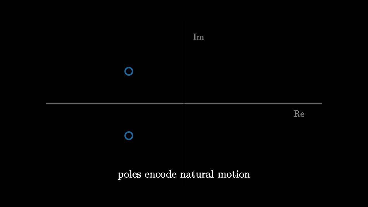
For more complicated linear systems, the denominator of the Laplace-domain expression encodes the modes of the system. Poles tell you whether responses decay, oscillate, or grow.

This is why engineers draw pole-zero diagrams. They are not decorative. They are maps of the system's possible behaviors.

Convolution becomes multiplication

Linear time-invariant systems respond to inputs by convolution:

y(t)=\int_0^t h(t-\tau)x(\tau)\,d\tau,

where $h$ is the impulse response. In the Laplace domain, this becomes

$$ Y(s)=H(s)X(s). $$

This is the same miracle as Fourier analysis. Complicated accumulation in time becomes multiplication after a transform. The transform chooses coordinates in which the system acts independently on each exponential mode.

Why exponentials are the right probes

The function $e^{st}$ is an eigenfunction of differentiation:

\frac{d}{dt}e^{st}=se^{st}.

That one equation explains the whole method. Linear differential equations are built from differentiation and addition. Exponentials turn differentiation into multiplication, so they diagonalize the behavior of the system.

The Laplace transform measures a signal against decaying exponentials because those are the shapes linear systems understand.

Seen this way, the transform is not a bag of table entries. It is a change of viewpoint. Time-domain behavior can be tangled, with memory and accumulation. In the Laplace domain, the same behavior becomes algebraic structure: poles, zeros, multiplication, and division.

The cost is abstraction. The reward is that a moving system becomes a static expression.