Monocurl Essays
Series Download

Elasticity: when raising the price lowers revenue

Revenue is a rectangle under the demand curve. Elasticity compares percentage changes in quantity and price, and decides whether a price rise grows it.

19 min·High school and early college·

AssumesSupply and demand: where a price comes fromWhat slope means, and why y = mx + b is a line

A cinema’s demand curve (left) and its nightly revenue (right). Revenue is the area of the shaded rectangle, price times tickets sold. As the price climbs from $4 the rectangle grows, then shrinks. It is largest, $3000, at a price of $10.
Monocurl source
let FA = Frame(0, 600, 0, 20, [-1.85, 0.15, 0], 2.7, 2.9)
let FR = Frame(0, 20, 0, 3200, [2.3, 0.15, 0], 2.6, 2.9)
let Shade = |p| RevBox(FA, p, tint(EMBER, 0.32))
let Dots = |p| [
    Pt(at(FA, Qd(p), p), EMBER, 0.1),
    Pt(at(FR, p, Rev(p)), EMBER, 0.1),
    center{at(FR, 12.5, 500)} color{EMBER} Number(Rev(p), 0)
]
mesh shade = Shade(p: 4)
mesh plots = [
    Plot(FA, [200, 400, 600], [5, 10, 15, 20], "tickets per night", "price ($ per ticket)", 0.95),
    Plot(FR, [5, 10, 15, 20], [1000, 2000, 3000], "price ($ per ticket)", "revenue ($ per night)", 1.0, 0.45)
]
mesh curves = [
    Demand(FA),
    Graph(FR, Rev, 0, 20, EMBER, 4)
]
mesh dots = Dots(p: 4)

slide "sweep"
    play Wait(0.6)
    shade.p = 16
    dots.p = 16
    play Lerp(5, [&shade, &dots], linear)
    play Wait(0.4)
    shade.p = 10
    dots.p = 10
    play Lerp(2.5, [&shade, &dots])
    play Wait(1.8)

Uses the shared definitions for this lesson's figures.

A cinema charges $8 a ticket. It raises the price to $10 and its nightly takings go up. A year later it raises the price again, from $12 to $14, and its takings go down. The hall, the films and the town are the same, and both increases were $2. Why did the second one backfire?

To have numbers to work with, suppose the number of tickets the town buys per night at a price of $P$ dollars is

$$ Q = 600 - 30P, \qquad 0 \le P \le 20. $$

One way such a formula arises, following the lesson on supply and demand: 600 residents each have a highest price they would pay for a ticket, those prices are spread evenly between $0 and $20, and so each extra dollar loses 30 customers. This is the cinema’s demand curve. It holds everything except the ticket price fixed, including incomes, the films on offer and the price of streaming at home.

Price $P$ (dollars)46810121416
Tickets $Q$480420360300240180120
Revenue $P \times Q$ (dollars)1920252028803000288025201920

The table reproduces the story. From $8 to $10 revenue rises from $2880 to $3000, and from $12 to $14 it falls from $2880 to $2520.

Revenue is a rectangle

On the demand graph, a price $P$ and the quantity $Q$ sold at it are the height and the width of a rectangle with one corner at the origin and the opposite corner on the curve. Revenue is its area. A price rise makes the rectangle taller and narrower, and the area changes by the difference of two strips.

  1. At 8 dollars the cinema sells 360 tickets. Revenue is the area of the rectangle, 2880 dollars.
  2. Raise the price to 10 dollars. Gained: 2 dollars more on each of 300 tickets. Lost: 60 tickets at 8 dollars each.
  3. Start again at 12 dollars, where 240 tickets sell. Revenue is again 2880 dollars.
  4. Raise the price to 14 dollars. Gained: 2 dollars more on each of 180 tickets. Lost: 60 tickets at 12 dollars each.
Raising the price trades one strip of revenue for another. The green strip is the extra $2 on every ticket still sold. The red strip is the tickets no longer sold, at the old price. From $8 the green strip is bigger; from $12 the red one is.
Monocurl source
let Words = |p0, p1| {
    let g = (p1 - p0) * Qd(p1)
    let l = p0 * (Qd(p0) - Qd(p1))
    var sgn = "{+}"
    if (g < l) { sgn = "{-}" }
    return [
        center{at(FD, 500, 17.5)} Math(str_join(["\text{gained } ", to_string(g, 0)]), 0.78, LEAF),
        center{at(FD, 500, 12.5)} Math(str_join(["\text{lost } ", to_string(l, 0)]), 0.78, ROSE),
        center{at(FD, 500, 7.5)} Math(str_join(["\text{net } ", sgn, to_string(abs(g - l), 0)]), 0.78, INK)
    ]
}
let Split = |p0, p1| [
    Strip(FD, 0, Qd(p1), 0, p0, tint(EMBER, 0.32)),
    Strip(FD, 0, Qd(p1), p0, p1, tint(LEAF, 0.5)),
    Strip(FD, Qd(p1), Qd(p0), 0, p0, tint(ROSE, 0.5))
]
let Area = |p| [center{at(FD, 500, 17.5)} Math(str_join([to_string(p, 0), " \times ", to_string(Qd(p), 0), " = ", to_string(Rev(p), 0)]), 0.78, EMBER)]
mesh fills = []
mesh plot = DemPlot(FD)
mesh demand = Demand(FD)
mesh notes = []

slide "At 8 dollars the cinema sells 360 tickets. Revenue is the area of the rectangle, 2880 dollars."
    fills = [RevBox(FD, 8, tint(EMBER, 0.32))]
    notes = Area(8)
    play Fade(0.6)

slide "Raise the price to 10 dollars. Gained: 2 dollars more on each of 300 tickets. Lost: 60 tickets at 8 dollars each."
    notes = []
    play Fade(0.3, [&notes])
    fills = Split(8, 10)
    notes = Words(8, 10)
    play Fade(0.6)

slide "Start again at 12 dollars, where 240 tickets sell. Revenue is again 2880 dollars."
    notes = []
    fills = []
    play Fade(0.3)
    fills = [RevBox(FD, 12, tint(EMBER, 0.32))]
    notes = Area(12)
    play Fade(0.6)

slide "Raise the price to 14 dollars. Gained: 2 dollars more on each of 180 tickets. Lost: 60 tickets at 12 dollars each."
    notes = []
    play Fade(0.3, [&notes])
    fills = Split(12, 14)
    notes = Words(12, 14)
    play Fade(0.6)

Uses the shared definitions for this lesson's figures.

Pause and try

Before stepping to the last slide, compute both strips for the rise from $12 to $14 yourself. How many tickets are still sold, and what does each bring in extra? How many are lost, and what did each bring in before?

Show answerHide answer

At $14 the cinema sells 180 tickets, each bringing $2 more than before: the gain is $2 \times 180 = 360$ dollars. It loses $240 - 180 = 60$ tickets that used to bring $12 each: the loss is $12 \times 60 = 720$ dollars. The net change is $360 - 720 = -360$, matching $2520 - 2880$.

So the question “does a higher price raise revenue?” is a contest between two strips. The gain is the price change times the quantity that remains. The loss is the quantity change times the old price.

Slope does not settle the contest

The natural first idea is that the outcome depends on how steep the demand curve is, meaning how many customers each extra dollar drives away. That idea fails on the spot, because the cinema’s demand is a straight line. Its slope is the same everywhere: 30 tickets lost per dollar, at $8 and at $12 alike.

Slope has a second defect. Its value depends on the units. Quote the price in cents and the same demand curve reads $Q = 600 - 0.3c$, with a slope of $0.3$ tickets per cent. Whether a price rise pays cannot depend on the currency unit, so the deciding quantity must be one that ignores units. Percentages do.

Price changeChange in priceChange in tickets
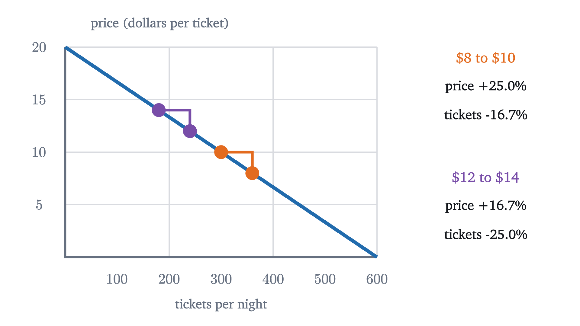
$8 to $10$+2$ on 8, or $+25\%$$-60$ on 360, or $-16.7\%$
$12 to $14$+2$ on 12, or $+16.7\%$$-60$ on 240, or $-25\%$
Two $2 price rises on the same straight demand line. The slope triangles are identical, but as percentages the first is a large price rise with a small loss of customers, and the second is the reverse.
Monocurl source
let Tri = |p, col| [
    Path([at(FN, Qd(p), p), at(FN, Qd(p), p + 2), at(FN, Qd(p + 2), p + 2)], col, 3.5),
    Pt(at(FN, Qd(p), p), col, 0.09),
    Pt(at(FN, Qd(p + 2), p + 2), col, 0.09)
]
let Pct = |y, p, col| [
    center{[2.7, y, 0]} Cap(str_join(["$", to_string(p, 0), " to $", to_string(p + 2, 0)]), 0.78, col),
    center{[2.7, y - 0.4, 0]} Cap(str_join(["price +", to_string(200 / p, 1), "%%"]), 0.74, INK),
    center{[2.7, y - 0.78, 0]} Cap(str_join(["tickets -", to_string(6000 / Qd(p), 1), "%%"]), 0.74, INK)
]
mesh plot = DemPlot(FN)
mesh demand = Demand(FN)
mesh tris = [Tri(8, EMBER), Tri(12, PLUM)]
mesh words = [Pct(1.45, 8, EMBER), Pct(-0.2, 12, PLUM)]

Uses the shared definitions for this lesson's figures.

Revenue is a product, and a product responds to proportional changes in its factors. At $8 the price rose by a quarter while the audience shrank by a sixth, and the product grew. At $12 the proportions were the other way round. The quantity we need is the ratio of the two percentages.

Elasticity

Before defining that ratio, one flaw in ordinary percentages has to be repaired. Going from $8 to $10 is a rise of 25 percent, but going back from $10 to $8 is a fall of 20 percent, because the base changed. A measure of how responsive buyers are between two points on the curve should not depend on which point we call the start. The standard repair is to measure each change against the average of its two values.

The numerator is the proportional change in quantity and the denominator is the proportional change in price. Units cancel in each, so $\varepsilon$ is a pure number. On a downward-sloping demand curve the two changes have opposite signs, so $\varepsilon$ is negative; many books quote only its size, $|\varepsilon|$. For the cinema:

$$ \text{from \$8 to \$10:}\quad \varepsilon = \frac{-60/330}{2/9} = -\frac{9}{11} \approx -0.82, \qquad \text{from \$12 to \$14:}\quad \varepsilon = \frac{-60/210}{2/13} = -\frac{13}{7} \approx -1.86. $$

Pause and try

Compute the midpoint elasticity for a price rise from $9 to $11 at the cinema, and the revenue at each of the two prices. What do you notice?

Show answerHide answer

The quantities are $600 - 270 = 330$ and $600 - 330 = 270$, so $\bar Q = 300$ and $\bar P = 10$. Then $\varepsilon = \dfrac{-60/300}{2/10} = \dfrac{-0.2}{0.2} = -1$. The revenues are $9 \times 330 = 2970$ and $11 \times 270 = 2970$: no change at all, at an elasticity of exactly $-1$.

Demand was inelastic where the price rise paid, elastic where it backfired, and unit elastic where it made no difference. That is a theorem, and the midpoint averages are what make it exact.

The middle line of the proof is the two strips again, each measured at an average: $(P_2 - P_1)\bar Q$ is the gain from the higher price and $(Q_2 - Q_1)\bar P$ is the (negative) loss from the lost sales. As a check, $2 \times 330 \times (1 - \frac{9}{11}) = 120$ and $2 \times 210 \times (1 - \frac{13}{7}) = -360$, the two revenue changes in the table.

The theorem assumed nothing about the shape of the demand curve. It holds for any two points with positive prices and quantities.

Elasticity at a single price

The midpoint formula needs two points. Often we want the elasticity at a price, for small changes around it. Take the cinema’s prices $P$ and $P + h$. The quantity changes by $-30h$, the average price is $P + \frac{h}{2}$, and the average quantity is $600 - 30P - 15h$, so

$$ \varepsilon = \frac{-30h}{600 - 30P - 15h} \cdot \frac{P + \frac h2}{h} = -30 \cdot \frac{P + \frac h2}{600 - 30(P + \frac h2)}. $$

That is $-30$ times price over quantity, evaluated at the midpoint. As $h$ shrinks toward 0 it approaches $-30P/Q$.

For the cinema, $\varepsilon(P) = -30P/(600 - 30P) = -P/(20 - P)$.

Pause and try

Compute the cinema’s point elasticity at $5, $10 and $15. The slope is the same at all three. What is changing?

Show answerHide answer

$\varepsilon(5) = -5/15 \approx -0.33$, $\varepsilon(10) = -10/10 = -1$, and $\varepsilon(15) = -15/5 = -3$. The slope factor, $-30$, is fixed, but it is multiplied by $P/Q$. Moving up the line, $P$ grows and $Q$ shrinks, so a dollar becomes a smaller fraction of the price while 30 tickets become a larger fraction of the audience.

The point elasticity along the cinema’s demand line. Its size is the price (orange part of the left edge) divided by the gap between the price and $20 (purple part). It is below 1 on the lower half of the line, exactly 1 at the middle, and grows without bound toward the top.
Monocurl source
let Along = |p| [
    Seg(at(FN, 0, 0), at(FN, 0, p), EMBER, 8),
    Seg(at(FN, 0, p), at(FN, 0, 20), PLUM, 8),
    stroke{SLATE, 2} dashed{[0.1, 0.08]} Line(at(FN, 0, p), at(FN, Qd(p), p)),
    Pt(at(FN, Qd(p), p), INK, 0.11),
    center{[2.7, 1.5, 0]} Note("price ($)", 0.74),
    center{[2.7, 1.08, 0]} scale{1.25} color{INK} Number(p, 1),
    center{[2.7, 0.3, 0]} Note("elasticity", 0.74),
    center{[2.7, -0.12, 0]} scale{1.25} color{INK} Number(-p / (20 - p), 2)
]
mesh plot = DemPlot(FN)
mesh demand = Demand(FN)
mesh names = [
    Pt(at(FN, 300, 10), LEAF, 0.1),
    center{at(FN, 300, 17.5)} Cap("elastic", 0.74, PLUM),
    center{at(FN, 500, 7.5)} Cap("inelastic", 0.74, EMBER),
    center{[2.7, -1.15, 0]} Math("\varepsilon = -\frac{P}{20 - P}", 1.0, SLATE)
]
mesh along = Along(p: 2)

slide "climb"
    play Wait(0.6)
    along.p = 18
    play Lerp(6, [&along], linear)
    play Wait(0.5)
    along.p = 10
    play Lerp(2, [&along])
    play Wait(1.6)

Uses the shared definitions for this lesson's figures.

This is why slope and elasticity must be kept apart. One straight line, with one slope, has every elasticity from nearly 0 at the bottom to arbitrarily large at the top.

For a straight line we can now say exactly where revenue peaks.

For the cinema, $a = 600$ and $b = 30$: the peak is at $P = 10$ with $R = 360000/120 = 3000$, as in the table. Readers who know calculus can reach the same place for any demand curve: $R'(P) = Q + PQ'(P) = Q\,(1 + \varepsilon)$, which is zero where $\varepsilon = -1$, and a maximum requires a zero slope. One caution about what this result means. Maximum revenue is not maximum profit, since tickets also cost something to provide; the next lesson deals with that.

Three special demand curves

A straight line passes through every elasticity. Three curves have the same elasticity everywhere, and they mark the limits of the definition.
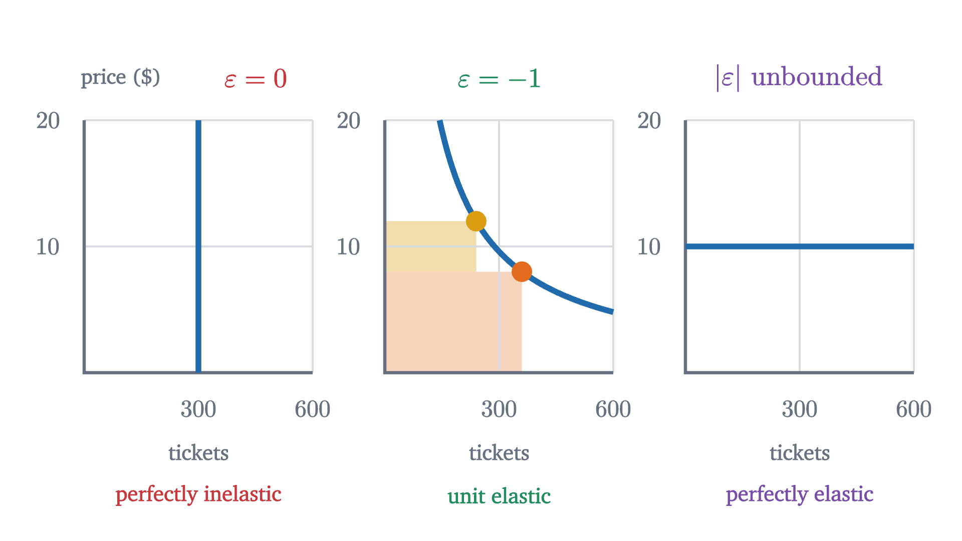
Demand curves with constant elasticity. A vertical curve: quantity ignores price. The curve Q = 2880/P: every rectangle under it has area 2880, so revenue never changes. A horizontal curve: any price above $10 loses every customer.
Demand curves with constant elasticity. A vertical curve: quantity ignores price. The curve $Q = 2880/P$: every rectangle under it has area 2880, so revenue never changes. A horizontal curve: any price above $10 loses every customer.
Monocurl source
let Mini = |i| Frame(0, 600, 0, 20, [-2.35 + 2.5 * i, 0.2, 0], 1.9, 2.1)
let Furniture = |i, title, verdict, col, tx = 300| {
    let f = Mini(i)
    return [
        Plot(f, [300, 600], [10, 20], "tickets", "", 0.5, 0.3),
        center{[fx(f, tx), fy(f, 20) + 0.35, 0]} Math(title, 0.82, col),
        center{[fx(f, 300), fy(f, 0) - 1.02, 0]} Cap(verdict, 0.72, col)
    ]
}
mesh boxes = [
    Strip(Mini(1), 0, 360, 0, 8, tint(EMBER, 0.3)),
    Strip(Mini(1), 0, 240, 8, 12, tint(GOLD, 0.35))
]
mesh panels = [
    Furniture(0, "\varepsilon = 0", "perfectly inelastic", ROSE, 450),
    Furniture(1, "\varepsilon = -1", "unit elastic", LEAF),
    Furniture(2, "|\varepsilon| \text{ unbounded}", "perfectly elastic", PLUM),
    center{[fx(Mini(0), 0) + 0.3, fy(Mini(0), 20) + 0.35, 0]} Note("price ($)", 0.7)
]
mesh curves = [
    Seg(at(Mini(0), 300, 0), at(Mini(0), 300, 20), AZURE, 4.5),
    stroke{AZURE, 4.5} Polyline(map(sample(4.8, 20, 60), |p| at(Mini(1), 2880 / p, p))),
    Pt(at(Mini(1), 360, 8), EMBER, 0.08),
    Pt(at(Mini(1), 240, 12), GOLD, 0.08),
    Seg(at(Mini(2), 0, 10), at(Mini(2), 600, 10), AZURE, 4.5)
]

Uses the shared definitions for this lesson's figures.

A vertical demand curve has $Q_2 = Q_1$ for every price change, so $\varepsilon = 0$: demand is perfectly inelastic, and a price rise raises revenue in full proportion. On the curve $Q = 2880/P$ revenue is $P \times Q = 2880$ at every price, so by the revenue test $1 + \varepsilon = 0$ between any two of its points: it is unit elastic everywhere. A horizontal demand curve has no elasticity under our definition, because the definition requires $P_1 \ne P_2$. It is the limiting case of flatter and flatter curves, on which $|\varepsilon|$ grows without bound, and it is called perfectly elastic. A wheat farmer who is one of thousands faces demand of this kind: at the market price she can sell all she has, and a cent above it, nothing.

What makes demand elastic

Elasticity is a property of buyers, and it has to be measured. The model does not tell us whether the demand for gasoline is elastic. Statistical studies do, and they find regular patterns. Demand tends to be more elastic when close substitutes exist (one brand of cereal against cereal in general), when the good takes a large share of the buyer’s budget, and when buyers have more time to adjust.
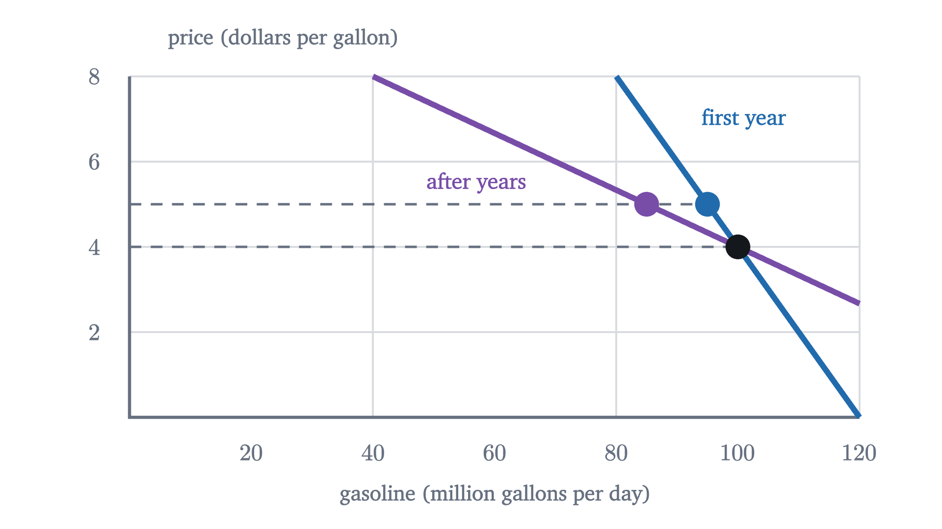
An illustration of the time horizon with made-up but typical numbers. Gasoline sells 100 million gallons a day at $4. If the price rises to $5, sales fall to 95 at first (elasticity about -0.2) and to 85 after some years (about -0.7), as drivers change cars and commutes.
An illustration of the time horizon with made-up but typical numbers. Gasoline sells 100 million gallons a day at $4. If the price rises to $5, sales fall to 95 at first (elasticity about $-0.2$) and to 85 after some years (about $-0.7$), as drivers change cars and commutes.
Monocurl source
let FG = Frame(0, 120, 0, 8, [0.2, 0.15, 0], 6.2, 2.9)
mesh plot = Plot(FG, [20, 40, 60, 80, 100, 120], [2, 4, 6, 8], "gasoline (million gallons per day)", "price (dollars per gallon)", 1.3, 0.3, [40, 80, 120])
mesh lines = [
    Seg(at(FG, 120, 0), at(FG, 80, 8), AZURE, 4.5),
    Seg(at(FG, 120, 8 / 3), at(FG, 40, 8), PLUM, 4.5),
    stroke{SLATE, 2} dashed{[0.1, 0.08]} Line(at(FG, 0, 5), at(FG, 95, 5)),
    stroke{SLATE, 2} dashed{[0.1, 0.08]} Line(at(FG, 0, 4), at(FG, 100, 4))
]
mesh dots = [
    Pt(at(FG, 100, 4), INK, 0.1),
    Pt(at(FG, 95, 5), AZURE, 0.1),
    Pt(at(FG, 85, 5), PLUM, 0.1)
]
mesh labels = [
    center{at(FG, 101, 7)} Cap("first year", 0.74, AZURE),
    center{at(FG, 57, 5.5)} Cap("after years", 0.74, PLUM)
]

Uses the shared definitions for this lesson's figures.

Surveys of the many studies of gasoline put its elasticity at roughly $-0.1$ to $-0.3$ in the short run (recent U.S. estimates are smaller, nearer $-0.05$) and two or three times that size over many years. Within a month a driver can only skip trips, but over several years she can buy a smaller car or move closer to work. These figures are estimates with wide error bands and they differ between places and periods. Treat any single quoted elasticity as approximate.

Two applications
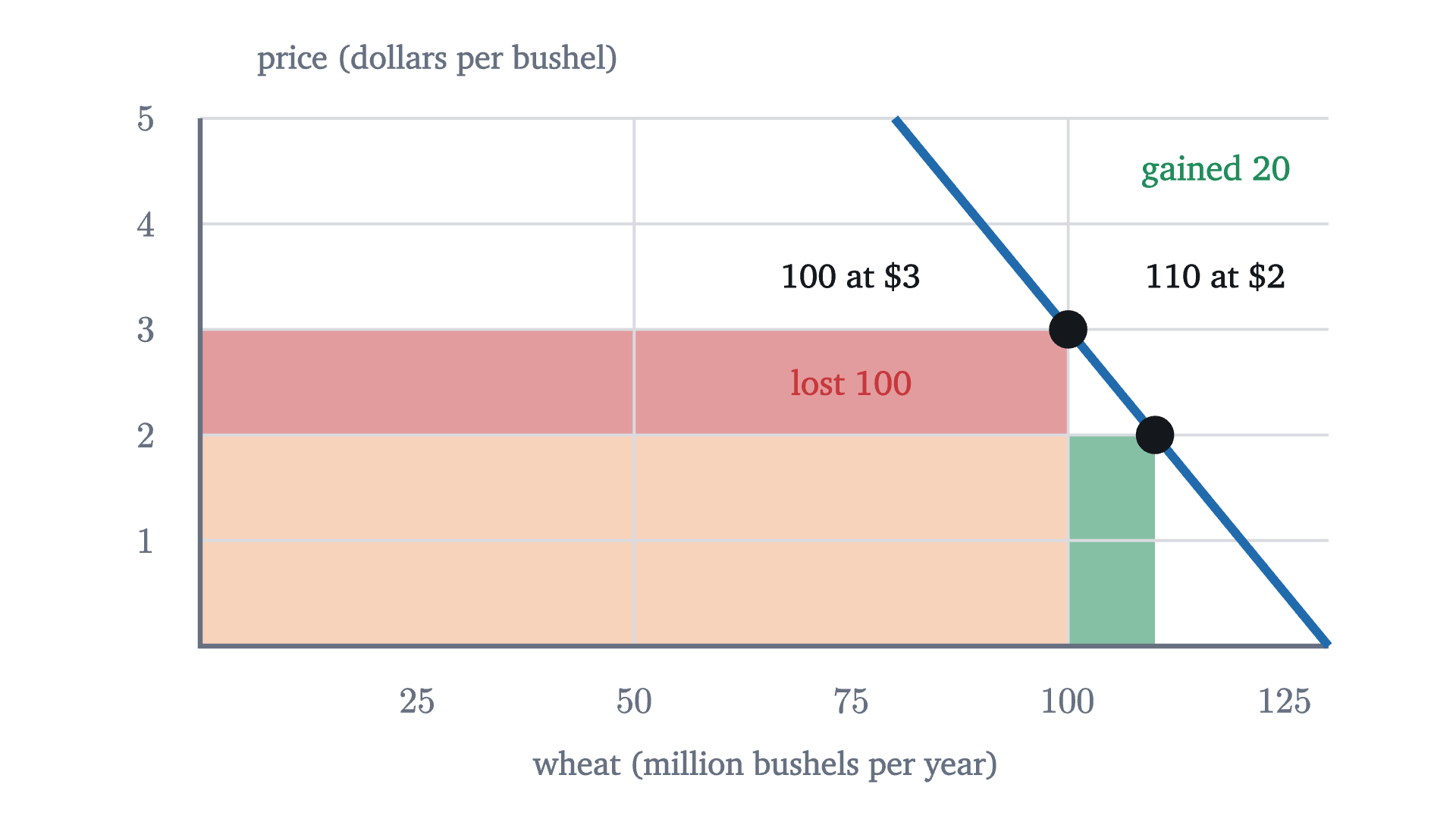
The wheat market in a normal year (100 million bushels at $3) and a bumper year (110 million at $2). Farmers gain the narrow green strip, 20 million dollars, and lose the wide red one, 100 million.
Monocurl source
let FW = Frame(0, 130, 0, 5, [0.2, 0.15, 0], 6.2, 2.9)
mesh fills = [
    Strip(FW, 0, 100, 0, 2, tint(EMBER, 0.3)),
    Strip(FW, 0, 100, 2, 3, tint(ROSE, 0.5)),
    Strip(FW, 100, 110, 0, 2, tint(LEAF, 0.55))
]
mesh plot = Plot(FW, [25, 50, 75, 100, 125], [1, 2, 3, 4, 5], "wheat (million bushels per year)", "price (dollars per bushel)", 1.3, 0.3, [50, 100])
mesh line = Seg(at(FW, 80, 5), at(FW, 130, 0), AZURE, 4.5)
mesh dots = [
    Pt(at(FW, 100, 3), INK, 0.1),
    Pt(at(FW, 110, 2), INK, 0.1)
]
mesh labels = [
    center{at(FW, 75, 2.5)} Cap("lost 100", 0.76, ROSE),
    center{at(FW, 117, 4.5)} Cap("gained 20", 0.76, LEAF),
    center{at(FW, 75, 3.5)} Cap("100 at $3", 0.74, INK),
    center{at(FW, 117, 3.5)} Cap("110 at $2", 0.74, INK)
]

Uses the shared definitions for this lesson's figures.

Check yourself

A museum finds that the elasticity of demand for its tickets is about $-0.6$ around the current price. If the only goal is more ticket revenue, what should it do?

What took the work here was finding the right measure. Slope was the obvious candidate and failed twice, and the measure that survived is the one the revenue rectangle itself picks out: the ratio of proportional changes, with midpoint averages. The same ratio can be formed for supply, and in the lesson on taxes the two responsiveness measures together decide who bears a tax.

Problems

The first three are direct computations, the next three need the theorems or an explanation, and the last two go further.

Problem 1

A café raises the price of a coffee from $4 to $5 and daily sales fall from 220 cups to 180. Compute the midpoint elasticity. Is demand elastic or inelastic over this range? Confirm with the revenues.

Show solutionHide solution

$\bar Q = 200$ and $\bar P = 4.5$. So $\varepsilon = \dfrac{-40/200}{1/4.5} = -0.2 \times 4.5 = -0.9$. Since $|\varepsilon| < 1$, demand is inelastic and the price rise should raise revenue. It does: $4 \times 220 = 880$ dollars before and $5 \times 180 = 900$ after. The revenue test gives the same change: $1 \times 200 \times (1 - 0.9) = 20$.

Problem 2

For the cinema, $Q = 600 - 30P$, find the point elasticity at prices of $4, $12 and $16, and say in each case which way revenue moves if the price is raised slightly.

Show solutionHide solution

$\varepsilon(P) = -P/(20 - P)$. At $4: $-4/16 = -0.25$, inelastic, revenue rises. At $12: $-12/8 = -1.5$, elastic, revenue falls. At $16: $-16/4 = -4$, elastic, revenue falls. This agrees with the table, where revenue climbs up to $10 and declines after it.

Problem 3

Demand for a ferry crossing is $Q = 80 - 4P$ passengers per trip, with $P$ in dollars. Find the price that maximizes revenue, the revenue there, and the point elasticity at that price.

Show solutionHide solution

Here $a = 80$ and $b = 4$, so the revenue-maximizing price is $\frac{a}{2b} = 10$ dollars. Then $Q = 80 - 40 = 40$ and $R = 400$ dollars, which matches $\frac{a^2}{4b} = \frac{6400}{16} = 400$. The elasticity is $-4 \times 10/40 = -1$, as the theorem requires.

Problem 4

A city bus carries 9000 riders a day at a fare of $2.00. The fare will rise to $2.50, and studies suggest a midpoint elasticity of $-0.4$ over this range. Predict the direction of the change in fare revenue without computing, then estimate the new ridership and revenue.

Show solutionHide solution

Demand is inelastic, so by the revenue test a fare rise increases revenue. For the size: $\bar P = 2.25$, so the proportional price change is $0.5/2.25 = \frac{2}{9}$ and the proportional quantity change is $-0.4 \times \frac29 = -\frac{4}{45}$. Solve $\dfrac{Q_2 - 9000}{(Q_2 + 9000)/2} = -\dfrac{4}{45}$: this gives $45(Q_2 - 9000) = -2(Q_2 + 9000)$, so $47 Q_2 = 387000$ and $Q_2 \approx 8234$ riders. Revenue goes from $2 \times 9000 = 18000$ dollars to $2.5 \times 8234 \approx 20585$ dollars a day.

Problem 5

The cinema’s demand in cents is $Q = 600 - 0.3c$, where $c$ is the price in cents. Find the slope and the point elasticity at a price of 1000 cents, and compare with the values in dollars. What does the comparison show?

Show solutionHide solution

The slope is $-0.3$ tickets per cent, against $-30$ tickets per dollar: a different number for the same curve. The elasticity is $-0.3 \times 1000 / (600 - 300) = -300/300 = -1$, the same as $\varepsilon(10) = -1$ in dollars. Changing the unit of price multiplies $P$ by 100 and divides the slope by 100, and the product $b \times P$ is untouched. Elasticity describes the buyers; slope describes the buyers and the choice of units together.

Problem 6

Rank these from least elastic demand to most elastic and justify the order: (a) gasoline, over the next month; (b) gasoline, over the next ten years; (c) gasoline from one particular station on a street with four stations.

Show solutionHide solution

Least to most elastic: (a), (b), (c). Over a month, drivers have almost no way to use less fuel, so quantity barely responds. Over ten years they can change cars, homes and jobs, so the same price rise removes more demand. One station among four faces a nearly perfect substitute a few meters away: a small price rise sends most of its customers next door, so its own demand is highly elastic even though the market’s is not. The good is the same in all three; what differs is how easily buyers can avoid the higher price.

Problem 7

In the wheat example, $Q = 130 - 10P$. (a) Which harvest size would give farmers the largest total revenue, and what is that revenue? (b) Compare it with the normal harvest of 100. (c) Explain why no individual farmer would choose to grow less.

Show solutionHide solution

(a) Revenue as a function of price is $P(130 - 10P)$, which by the theorem peaks at $P = \frac{130}{20} = 6.5$ dollars, where $Q = 65$ million bushels and revenue is $6.5 \times 65 = 422.5$ million dollars. (b) A normal harvest of 100 earns 300 million. Farmers as a group would earn about 41 percent more by growing 35 percent less, because at 100 they are on the inelastic part of the demand curve. (c) Each farmer is a price-taker: her own output does not change the price, so every extra bushel she grows adds the full price to her revenue. The gain from a smaller total crop exists only if all restrict together, and each has a reason to break ranks.

Problem 8

Prove that on the demand curve $Q = k/P$, with $k > 0$, the midpoint elasticity between any two points is exactly $-1$, directly from the definition and without using the revenue test.

Show solutionHide solution

Let the points be $(P_1, k/P_1)$ and $(P_2, k/P_2)$ with $P_1 \ne P_2$. Then

$$ Q_2 - Q_1 = \frac{k}{P_2} - \frac{k}{P_1} = \frac{k(P_1 - P_2)}{P_1 P_2}, \qquad Q_1 + Q_2 = \frac{k(P_1 + P_2)}{P_1 P_2}. $$

So $\dfrac{Q_2 - Q_1}{\bar Q} = \dfrac{2(Q_2 - Q_1)}{Q_1 + Q_2} = \dfrac{2(P_1 - P_2)}{P_1 + P_2}$, while $\dfrac{P_2 - P_1}{\bar P} = \dfrac{2(P_2 - P_1)}{P_1 + P_2}$. Their ratio is $\dfrac{P_1 - P_2}{P_2 - P_1} = -1$. This agrees with the revenue test: revenue is $k$ at every point, so $R_2 - R_1 = 0$ forces $1 + \varepsilon = 0$.

Shared definitions used by this lesson's figures
# house kit: prepended to every essay figure after the std imports

# palette. AZURE and EMBER are the two actors, LEAF marks an answer, ROSE a problem
let PAPER = [1, 1, 1, 1]
let INK = [0.08, 0.09, 0.11, 1]
let SLATE = [0.40, 0.44, 0.50, 1]
let MIST = [0.85, 0.86, 0.88, 1]
let AZURE = [0.13, 0.42, 0.68, 1]
let EMBER = [0.89, 0.42, 0.12, 1]
let LEAF = [0.13, 0.55, 0.36, 1]
let ROSE = [0.78, 0.22, 0.24, 1]
let PLUM = [0.47, 0.30, 0.66, 1]
let GOLD = [0.85, 0.62, 0.08, 1]

background = PAPER

# an opaque pastel of col; use for fills so overlaps do not darken
let tint = |col, amount = 0.18| [
    1 - (1 - col[0]) * amount,
    1 - (1 - col[1]) * amount,
    1 - (1 - col[2]) * amount,
    1
]

# text: Cap for labels, Note for quiet labels, Math for typeset maths
let Cap = |txt, size = 0.75, col = INK| color{col} Text(txt, size, "Charter")
let Note = |txt, size = 0.65| color{SLATE} Text(txt, size, "Charter")
let Math = |tex, size = 0.9, col = INK| color{col} Tex(tex, size)

# a paper rectangle to sit behind text that crosses lines
let Plate = |pos, size| center{pos} fill{PAPER} stroke{alpha{0} PAPER, 0} Rect(size)

# shapes with fill and stroke both set, so no stray black appears
let Pt = |pos, col = INK, r = 0.075| center{pos} fill{col} stroke{col, 1} Circle(r, 48)
let Ring = |pos, col = INK, r = 0.1, w = 3| center{pos} fill{PAPER} stroke{col, w} Circle(r, 48)
let Seg = |a, b, col = INK, w = 3| stroke{col, w} Line(a, b)
let Path = |pts, col = INK, w = 3| stroke{col, w} Polyline(pts)
let Region = |pts, col| fill{col} stroke{alpha{0} col, 0} Polygon(pts)
let Outline = |pts, col = INK, w = 3| fill{alpha{0} PAPER} stroke{col, w} Polygon(pts)
let Shape = |pts, col, amount = 0.18, w = 3| fill{tint(col, amount)} stroke{col, w} Polygon(pts)
let Disc = |pos, r, col, amount = 0.18, w = 3| center{pos} fill{tint(col, amount)} stroke{col, w} Circle(r, 96)
let Box = |pos, size, col, amount = 0.18, w = 3| center{pos} fill{tint(col, amount)} stroke{col, w} Rect(size)
# a line from a to b ending in a small solid arrowhead
let Tip = |a, b, col = INK, w = 3, head = 0.17| {
    let d = normalize([b[0] - a[0], b[1] - a[1], 0])
    let n = [-d[1], d[0], 0]
    let base = [b[0] - d[0] * head, b[1] - d[1] * head, 0]
    return [
        stroke{col, w} Line(a, base),
        fill{col} stroke{col, 1} Polygon([
            b,
            [base[0] + n[0] * head * 0.42, base[1] + n[1] * head * 0.42, 0],
            [base[0] - n[0] * head * 0.42, base[1] - n[1] * head * 0.42, 0]
        ])
    ]
}

# plots. a frame is [x0, x1, y0, y1, centre, width, height]: a data window and the scene box it fills
let Frame = |x0, x1, y0, y1, c = [0, 0, 0], w = 6.4, h = 3.6| [x0, x1, y0, y1, c, w, h]
let fx = |fr, x| fr[4][0] + (x - (fr[0] + fr[1]) / 2) * fr[5] / (fr[1] - fr[0])
let fy = |fr, y| fr[4][1] + (y - (fr[2] + fr[3]) / 2) * fr[6] / (fr[3] - fr[2])
let at = |fr, x, y| [fx(fr, x), fy(fr, y), 0]

# axes through the data origin (or the nearest edge of the window), with optional names
let Axes = |fr, x_name = "", y_name = "", col = SLATE| {
    let ox = clamp(fr[0], 0, fr[1])
    let oy = clamp(fr[2], 0, fr[3])
    var parts = [
        Tip(at(fr, fr[0], oy), [fx(fr, fr[1]) + 0.25, fy(fr, oy), 0], col, 2.5, 0.15),
        Tip(at(fr, ox, fr[2]), [fx(fr, ox), fy(fr, fr[3]) + 0.25, 0], col, 2.5, 0.15)
    ]
    if (x_name != "") {
        parts .= center{[fx(fr, fr[1]) + 0.5, fy(fr, oy), 0]} Math(x_name, 0.8, col)
    }
    if (y_name != "") {
        parts .= center{[fx(fr, ox), fy(fr, fr[3]) + 0.5, 0]} Math(y_name, 0.8, col)
    }
    return parts
}

# tick marks with numbers at the listed data values
let XTicks = |fr, xs, col = SLATE, places = 0| block {
    let oy = fy(fr, clamp(fr[2], 0, fr[3]))
    for (x in xs) {
        . Seg([fx(fr, x), oy - 0.07, 0], [fx(fr, x), oy + 0.07, 0], col, 2)
        . center{[fx(fr, x), oy - 0.33, 0]} Math(to_string(x, places), 0.72, col)
    }
}
let YTicks = |fr, ys, col = SLATE, places = 0| block {
    let ox = fx(fr, clamp(fr[0], 0, fr[1]))
    for (y in ys) {
        . Seg([ox - 0.07, fy(fr, y), 0], [ox + 0.07, fy(fr, y), 0], col, 2)
        . center{[ox - 0.36, fy(fr, y), 0]} Math(to_string(y, places), 0.72, col)
    }
}

# faint grid lines at the listed data values
let GridLines = |fr, xs, ys, col = MIST| block {
    for (x in xs) {
        . Seg(at(fr, x, fr[2]), at(fr, x, fr[3]), col, 1.5)
    }
    for (y in ys) {
        . Seg(at(fr, fr[0], y), at(fr, fr[1], y), col, 1.5)
    }
}

# the graph of f over [a, b], drawn in the frame. values are clamped to the window
let Graph = |fr, f, a, b, col = AZURE, w = 4, n = 160|
    stroke{col, w} Polyline(map(sample(a, b, n), |x| at(fr, x, clamp(fr[2], f(x), fr[3]))))

# the region between the graph of f and the x axis over [a, b]
let AreaUnder = |fr, f, a, b, col = AZURE, amount = 0.2, n = 80| {
    var pts = [at(fr, a, 0)]
    for (x in sample(a, b, n)) {
        pts .= at(fr, x, clamp(fr[2], f(x), fr[3]))
    }
    pts .= at(fr, b, 0)
    return fill{tint(col, amount)} stroke{alpha{0} col, 0} Polygon(pts)
}

# the cinema: tickets sold per night at a price of p dollars, and the night's revenue in dollars
let Qd = |p| 600 - 30 * p
let Rev = |p| p * Qd(p)
# plot furniture: grid, left and bottom edges, numbers along the edges, axis names
let Plot = |f, gx, gy, xname, yname, ynx = 1.0, ydx = 0.36, vx = nil| block {
    var vs = vx
    if (vx == nil) { vs = gx }
    . GridLines(f, vs, gy)
    . Path([at(f, f[0], f[3]), at(f, f[0], f[2]), at(f, f[1], f[2])], SLATE, 2.5)
    for (x in gx) {
        . center{[fx(f, x), fy(f, f[2]) - 0.3, 0]} Math(to_string(x, 0), 0.72, SLATE)
    }
    for (y in gy) {
        . center{[fx(f, f[0]) - ydx, fy(f, y), 0]} Math(to_string(y, 0), 0.72, SLATE)
    }
    . center{[(fx(f, f[0]) + fx(f, f[1])) / 2, fy(f, f[2]) - 0.66, 0]} Note(xname, 0.72)
    . center{[fx(f, f[0]) + ynx, fy(f, f[3]) + 0.32, 0]} Note(yname, 0.72)
}
let FD = Frame(0, 600, 0, 20, [0.2, 0.15, 0], 6.2, 2.9)
let FN = Frame(0, 600, 0, 20, [-0.95, 0.15, 0], 4.3, 2.9)
let DemPlot = |f| Plot(f, [100, 200, 300, 400, 500, 600], [5, 10, 15, 20], "tickets per night", "price (dollars per ticket)", 1.3, 0.36, [200, 400, 600])
let Demand = |f| Seg(at(f, 0, 20), at(f, 600, 0), AZURE, 4.5)
# a filled rectangle in data coordinates
let Strip = |f, q0, q1, p0, p1, col| Region([at(f, q0, p0), at(f, q1, p0), at(f, q1, p1), at(f, q0, p1)], col)
let RevBox = |f, p, col| Strip(f, 0, Qd(p), 0, p, col)