
Monocurl Essays
Series Download

Bayes' rule: why a positive test is usually a false alarm

A 99% accurate test for a rare disease comes back positive, and the chance you are sick is about 9%. Conditional probability and Bayes' theorem explain why.

22 min·High school and early college·

AssumesWhat probability means: counting equally likely outcomes

One thousand people, one of whom has the disease (orange). Everyone is tested. The test flags the sick person and also about 1% of the 999 healthy people, so of the 11 people with a positive result only 1 is sick.
Monocurl source
let COLS = 50
let ROWS = 20
let GAP = 0.14
let N = COLS * ROWS
let dot_pos = |i| [-3.43 + mod(i, COLS) * GAP, 1.95 - (i // COLS) * GAP, 0]
let n_sick = to_int(round(N * PREV))
let n_fp = to_int(round((N - n_sick) * FPR))
# pick which people are sick and which healthy people are flagged, by hashing
var chosen = []
var seed = 1
while (len(chosen) < n_sick + n_fp) {
    let i = to_int(floor(N * rnd(seed, 5)))
    if (not (i in chosen)) {
        chosen .= i
    }
    seed = seed + 1
}
let SICK = chosen[0]
let ORDER = sort(chosen)
let PALE = tint(AZURE, 0.5)
let sm = |x| {
    let u = clamp(0, x, 1)
    return u * u * (3 - 2 * u)
}
let Special = |s| {
    let scan_x = -3.6 + 7.2 * clamp(0, s - 1, 1)
    let fly = sm(s - 2)
    let done = sm((s - 3) * 2)
    let reveal = sm(s * 1.5)
    var parts = []
    for (r in range(0, len(ORDER))) {
        let home = dot_pos(ORDER[r])
        let hit = sm((scan_x - home[0]) * 5)
        var col = lerp(PALE, AZURE, fly)
        var rad = 0.045
        if (ORDER[r] == SICK) {
            col = lerp(PALE, EMBER, reveal)
            rad = 0.045 + 0.04 * reveal
        }
        let p = lerp(home, [-1.75 + r * 0.35, -1.25, 0], fly)
        let rr = rad + (0.1 - rad) * fly
        parts .= center{p} fill{col} stroke{col, 1} Circle(rr, 24)
        if (hit > 0.01) {
            parts .= center{p} fill{alpha{0} PAPER} stroke{alpha{hit} PLUM, 3} Circle(rr + 0.05, 24)
        }
    }
    let scan_a = sm((s - 1) * 8) * (1 - sm((s - 1.92) * 12))
    parts .= stroke{alpha{scan_a} PLUM, 3} Line([scan_x, 2.05, 0], [scan_x, -0.8, 0])
    parts .= center{[0, -1.85, 0]} Cap(str_join([to_string(N), " people, ", to_string(n_sick), " of them sick"]), 0.8, alpha{1 - sm((s - 2) * 3)} INK)
    parts .= center{[0, -1.85, 0]} Cap(str_join([to_string(n_sick + n_fp), " positive tests, ", to_string(n_sick), " sick person"]), 0.8, alpha{done} INK)
    return parts
}
mesh crowd = block {
    for (i in range(0, N)) {
        if (not (i in ORDER)) {
            . center{dot_pos(i)} fill{PALE} stroke{PALE, 1} Circle(0.045, 12)
        }
    }
}
mesh legend = [
    Pt([-3.4, -1.25, 0], EMBER, 0.085),
    center{[-2.9, -1.25, 0]} Cap("sick", 0.75, EMBER),
    center{[2.35, -1.25, 0]} fill{alpha{0} PAPER} stroke{PLUM, 3} Circle(0.1, 24),
    center{[3.05, -1.25, 0]} Cap("positive", 0.75, PLUM)
]
mesh special = Special(s: 0)

slide "test"
    play Wait(0.5)
    special.s = 1
    play Lerp(1.2, [&special], linear)
    play Wait(0.4)
    special.s = 2
    play Lerp(2.6, [&special], linear)
    play Wait(0.4)
    special.s = 3.5
    play Lerp(2.4, [&special], linear)
    play Wait(2)

Uses the shared definitions for this lesson's figures.

A disease affects one person in a thousand. There is a test for it that is 99% accurate: it gives the right answer for 99% of sick people and for 99% of healthy people. You take the test as part of a routine checkup, with no symptoms, and it comes back positive. What is the chance that you have the disease?

Pause and try

Write down your answer before reading further, as a percentage. Then try to justify it with a calculation.

Show answerHide answer

Most people answer 99% or something close to it, and in published studies many physicians have made the same mistake on similar screening problems. The correct answer is about 9%. The rest of this lesson explains where the missing 90 percentage points went.

The animation above shows where the 9% comes from. Take a thousand people. On average one of them is sick, and the test will almost certainly flag that person. But the test also errs on 1% of the 999 healthy people, which is about ten more positives. So there are about eleven positive results, and only one of them belongs to a sick person. You are one of the eleven, and you do not know which.

The 99% and the 9% are both correct. They answer different questions, and to tell the questions apart we need a way to say “the probability of this, given that”: conditional probability. Dice make it visible, so we start there.

New information shrinks the sample space

Recall the setup from the lesson on sample spaces. Rolling a blue die and an orange die has 36 equally likely outcomes, the pairs $(a, b)$ with $a$ the blue face and $b$ the orange face. An event is a set of outcomes, and when outcomes are equally likely its probability is the number of outcomes in it divided by 36. For example “doubles” (both dice the same) is 6 cells of the grid, so its probability is $6/36 = 1/6$.

Now suppose the dice are rolled where you cannot see them, and a friend who can see them tells you one thing: the total is at least 10.

Pause and try

Given that the total is at least 10, what is the probability that the roll is a double? List the outcomes that are still possible.

Show answerHide answer

A total of at least 10 leaves six outcomes: $(4,6), (5,5), (6,4), (5,6), (6,5), (6,6)$. Two of them, $(5,5)$ and $(6,6)$, are doubles. So the probability is $2/6 = 1/3$, twice what it was before your friend spoke.

  1. Before any information, doubles are 6 of the 36 equally likely cells.
  2. You learn that the total is at least 10. Thirty cells are now impossible and six remain.
  3. Among those six, two are doubles. Given the new information, the probability of doubles is 2/6.
Conditioning on the grid of 36 outcomes for two dice. Learning that the total is at least 10 removes thirty cells. The probability of doubles is then counted among the six that remain.
Monocurl source
let dbl = |a, b| a == b
let big = |a, b| a + b >= 10
let small = |a, b| a + b < 10
let n_dbl = count_cells(dbl)
let n_big = count_cells(big)
let n_both = count_cells(|a, b| a == b and a + b >= 10)
mesh base = [Headers, Lit(|a, b| 1, SLATE, 0.1)]
mesh hi = []
mesh ghost = []
mesh keep = []
mesh panel = []

slide "Before any information, doubles are 6 of the 36 equally likely cells."
    hi = Lit(dbl, EMBER)
    panel = [
        center{[2.1, 1.2, 0]} Cap("doubles", 0.9, EMBER),
        center{[2.1, 0.2, 0]} Frac(n_dbl, 36, 1.3, EMBER)
    ]
    play Fade(0.7)

slide "You learn that the total is at least 10. Thirty cells are now impossible and six remain."
    panel = []
    play Fade(0.3, [&panel])
    ghost = Lit(small, MIST, 0.25)
    keep = Outline([
        [GX + 6 * CELL, GY, 0], [GX + 6 * CELL, GY + 3 * CELL, 0], [GX + 5 * CELL, GY + 3 * CELL, 0],
        [GX + 5 * CELL, GY + 2 * CELL, 0], [GX + 4 * CELL, GY + 2 * CELL, 0], [GX + 4 * CELL, GY + CELL, 0],
        [GX + 3 * CELL, GY + CELL, 0], [GX + 3 * CELL, GY, 0]
    ], PLUM, 4)
    panel = [
        center{[2.1, 1.2, 0]} Cap("total at least 10", 0.9, PLUM),
        center{[2.1, 0.4, 0]} Cap(str_join([to_string(n_big), " cells remain"]), 0.82)
    ]
    play Fade(0.8)

slide "Among those six, two are doubles. Given the new information, the probability of doubles is 2/6."
    panel = []
    play Fade(0.3, [&panel])
    panel = [
        center{[2.1, 1.45, 0]} Cap("doubles, given", 0.85, EMBER),
        center{[2.1, 1.0, 0]} Cap("total at least 10", 0.85, PLUM),
        center{[2.1, -0.1, 0]} Frac(n_both, n_big, 1.3, EMBER),
        center{[2.1, -1.3, 0]} Cap(str_join(["it was ", to_string(n_dbl), " of 36"]), 0.8, SLATE)
    ]
    play Fade(0.6, [&panel])

Uses the shared definitions for this lesson's figures.

Look at what the calculation did. The information “total at least 10” is an event, call it $B$, with 6 cells. Once we know $B$ occurred, the outcomes outside $B$ are impossible, and the outcomes inside $B$ are still equally likely among themselves, since nothing we learned favors one of them over another. So $B$ becomes the new sample space. The event $A$ = “doubles” survives only as the part of it inside $B$, which is $A \cap B$, and

$$ \frac{|A \cap B|}{|B|} = \frac{2}{6}. $$

Divide the top and bottom by 36 and the same number reads $\frac{2/36}{6/36} = \frac{P(A \cap B)}{P(B)}$. In that form it no longer mentions counting, so it makes sense for any probability measure, and it is taken as the definition.

The hypothesis $P(B) > 0$ is there because we divide by $P(B)$; we cannot condition on something that has no chance of happening. The numerator is the part of $A$ compatible with what we learned. The denominator rescales so that the new sample space $B$ has total probability 1: indeed $P(B \mid B) = 1$.

Multiplying through by $P(B)$ gives a form that is often more useful, the multiplication rule:

$$ P(A \cap B) = P(A \mid B)\, P(B). $$

In words: for both to happen, $B$ must happen, and then $A$ must happen given that $B$ did.

The order matters

Conditional probability has a trap built into its notation, and the opening question walks straight into it. Compute the dice example the other way round: given that the roll is a double, what is the probability that the total is at least 10? Now the new sample space is the 6 doubles, and 2 of them have a total of at least 10, so $P(B \mid A) = 2/6$ as well. The two agree here only because $A$ and $B$ happen to have the same size. Change the event to see them come apart. Let $C$ be “the total is 12”, the single cell $(6,6)$. Then

$$ P(C \mid A) = \frac{1}{6}, \qquad P(A \mid C) = \frac{1}{1} = 1. $$

Given a double, a 12 is unlikely. Given a 12, a double is certain. Both fractions have the same numerator, $P(A \cap C) = 1/36$, and different denominators, because they are fractions of different sets.

Return to the test with this in mind. Write $S$ for “the person is sick” and $+$ for “the test is positive”. The accuracy figure quoted for the test is $P(+ \mid S) = 0.99$: of the sick, the fraction who test positive. The question you care about after a positive result is $P(S \mid +)$: of those who test positive, the fraction who are sick. These are fractions of different groups of people, and the hero animation showed how different the groups are. Almost all sick people are in the positive group, and yet the positive group is mostly healthy people, because there were so many healthy people to begin with.

Counting the positives exactly

The thousand-person picture rounded a little: 1% of 999 is 9.99 people. To get exact whole numbers, imagine 100,000 people instead and follow them through the test. We need three numbers about the test and the population, and it is worth giving each its standard name. The prevalence is $P(S) = 0.001$. The sensitivity is $P(+ \mid S) = 0.99$. The false positive rate is $P(+ \mid S^c) = 0.01$, where $S^c$ is the complement of $S$, “the person is healthy”.

  1. Of 100,000 people who take the test, one in a thousand is sick: 100 people. The other 99,900 are healthy.
  2. The test is positive for 99 of every 100 sick people. It misses 1.
  3. It is also positive for 1 of every 100 healthy people: 999 people, far more than the 99.
  4. Collect the positives: 99 + 999 = 1098. The sick are 99 of them, about 1 in 11.
One hundred thousand people followed through the test. The sick and the healthy are each split by their test result, and the positives from both branches are collected at the end.
Monocurl source
let NPOP = 100000
let n_sick = NPOP * PREV
let n_well = NPOP - n_sick
let tp = n_sick * SENS
let fp = n_well * FPR
let Node = |pos, num, label, col, w = 1.65| [
    Box(pos, [w, 0.8], col, 0.14, 3),
    center{[pos[0], pos[1] + 0.17, 0]} Cap(commas(num), 0.85, col),
    center{[pos[0], pos[1] - 0.2, 0]} Cap(label, 0.7, col)
]
let ROOT = [0, 1.6, 0]
let PS = [-1.9, 0.45, 0]
let PW = [1.9, 0.45, 0]
let LEAVES = [[-2.8, -0.7, 0], [-1.0, -0.7, 0], [1.0, -0.7, 0], [2.8, -0.7, 0]]
let Link = |a, b| Seg([a[0], a[1] - 0.4, 0], [b[0], b[1] + 0.4, 0], SLATE, 2.5)
let Halo = |pos| Outline([
    [pos[0] - 0.9, pos[1] - 0.47, 0], [pos[0] + 0.9, pos[1] - 0.47, 0],
    [pos[0] + 0.9, pos[1] + 0.47, 0], [pos[0] - 0.9, pos[1] + 0.47, 0]
], PLUM, 5)
mesh links = []
mesh root = Node(ROOT, NPOP, "people", INK, 2.0)
mesh level1 = []
mesh sick_leaves = []
mesh well_leaves = []
mesh halo = []
mesh result = []

slide "Of 100,000 people who take the test, one in a thousand is sick: 100 people. The other 99,900 are healthy."
    links = [Link(ROOT, PS), Link(ROOT, PW)]
    level1 = [
        Node(PS, n_sick, "sick", EMBER),
        Node(PW, n_well, "healthy", AZURE),
        center{[-1.75, 1.15, 0]} Note("0.1%%", 0.72),
        center{[1.75, 1.15, 0]} Note("99.9%%", 0.72)
    ]
    play Fade(0.7)

slide "The test is positive for 99 of every 100 sick people. It misses 1."
    links .= Link(PS, LEAVES[0])
    links .= Link(PS, LEAVES[1])
    sick_leaves = [
        Node(LEAVES[0], tp, "positive", EMBER),
        Node(LEAVES[1], n_sick - tp, "negative", EMBER),
        center{[-2.85, -0.1, 0]} Note("99%%", 0.72),
        center{[-0.95, -0.1, 0]} Note("1%%", 0.72)
    ]
    play Fade(0.7)

slide "It is also positive for 1 of every 100 healthy people: 999 people, far more than the 99."
    links .= Link(PW, LEAVES[2])
    links .= Link(PW, LEAVES[3])
    well_leaves = [
        Node(LEAVES[2], fp, "positive", AZURE),
        Node(LEAVES[3], n_well - fp, "negative", AZURE),
        center{[0.95, -0.1, 0]} Note("1%%", 0.72),
        center{[2.85, -0.1, 0]} Note("99%%", 0.72)
    ]
    play Fade(0.7)

slide "Collect the positives: 99 + 999 = 1098. The sick are 99 of them, about 1 in 11."
    halo = [Halo(LEAVES[0]), Halo(LEAVES[2])]
    result = center{[0, -1.72, 0]} Math(str_join([
        "\frac{", commas(tp), "}{", commas(tp), " + ", commas(fp), "} = \frac{", commas(tp), "}{", commas(tp + fp, "{,}"), "} \approx ", to_string(tp / (tp + fp), 3)
    ]), 1.0)
    play Fade(0.8)

Uses the shared definitions for this lesson's figures.

Of 100,000 people, 1098 test positive, and 99 of those are sick. So

$$ P(S \mid +) = \frac{99}{1098} \approx 0.090. $$

A positive result has moved your chance of being sick from 1 in 1000 to about 1 in 11. That is a ninety-fold increase, and the test deserves credit for it. It is still far from 99%, and the reason is in the tree: the healthy branch is 999 times as wide as the sick branch, so even a 1% error rate on it produces about ten times as many positives as the whole sick branch can.

The same computation as areas

The tree used 100,000 people for convenience, and nothing depended on that number. To see the structure without a population, draw the sample space as a square of area 1 and let area stand for probability. I would like to draw the disease this way, but a strip for the sick one-thousandth as wide as the square would be invisible, which is itself a fair picture of the problem. So here is a test with friendlier proportions. Among children brought to a clinic with a sore throat, suppose 30% have strep. A rapid strep test is positive for 85% of those who have it and for 5% of those who do not.
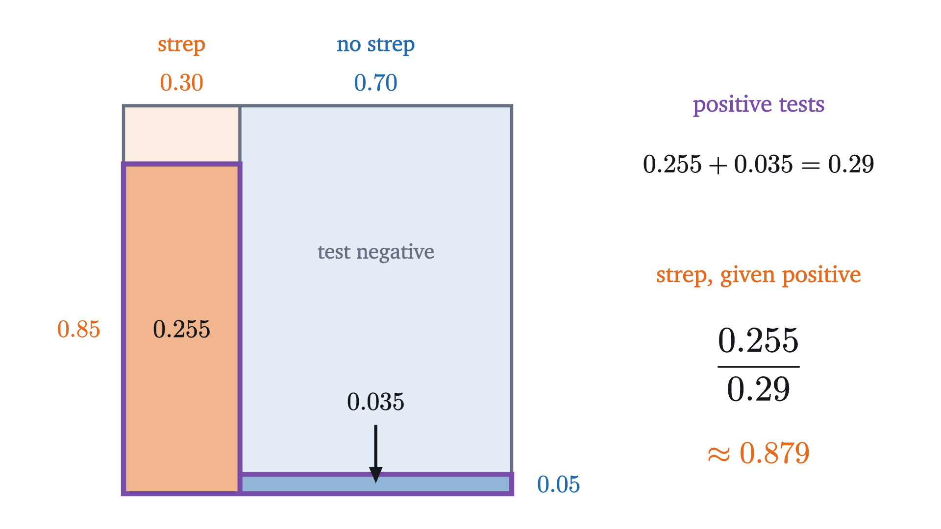
Bayes' rule as areas, for the strep test. The square has area 1. Its width is split by who has strep (30%) and who does not (70%), and each column is split by height according to how often the test is positive in that group. The positive results are the two outlined rectangles, and the chance of strep given a positive is the orange rectangle's share of their combined area.
Bayes’ rule as areas, for the strep test. The square has area 1. Its width is split by who has strep (30%) and who does not (70%), and each column is split by height according to how often the test is positive in that group. The positive results are the two outlined rectangles, and the chance of strep given a positive is the orange rectangle’s share of their combined area.
Monocurl source
let P_H = 0.3
let S_H = 0.85
let F_H = 0.05
let W = 3.3
let X0 = -2.95
let Y0 = -1.95
let xs = X0 + P_H * W
let a_sick = P_H * S_H
let a_well = (1 - P_H) * F_H
let Rc = |x0, x1, y0, y1| [[x0, y0, 0], [x1, y0, 0], [x1, y1, 0], [x0, y1, 0]]
mesh fills = [
    Region(Rc(X0, xs, Y0, Y0 + W), tint(EMBER, 0.12)),
    Region(Rc(xs, X0 + W, Y0, Y0 + W), tint(AZURE, 0.12)),
    Region(Rc(X0, xs, Y0, Y0 + S_H * W), tint(EMBER, 0.5)),
    Region(Rc(xs, X0 + W, Y0, Y0 + F_H * W), tint(AZURE, 0.5))
]
mesh lines = [
    Outline(Rc(X0, X0 + W, Y0, Y0 + W), SLATE, 2.5),
    Seg([xs, Y0, 0], [xs, Y0 + W, 0], SLATE, 2.5),
    Outline(Rc(X0, xs, Y0, Y0 + S_H * W), PLUM, 4),
    Outline(Rc(xs, X0 + W, Y0, Y0 + F_H * W), PLUM, 4)
]
mesh labels = [
    center{[(X0 + xs) / 2, Y0 + W + 0.5, 0]} Cap("strep", 0.75, EMBER),
    center{[(X0 + xs) / 2, Y0 + W + 0.2, 0]} Math(to_string(P_H, 2), 0.75, EMBER),
    center{[(xs + X0 + W) / 2, Y0 + W + 0.5, 0]} Cap("no strep", 0.75, AZURE),
    center{[(xs + X0 + W) / 2, Y0 + W + 0.2, 0]} Math(to_string(1 - P_H, 2), 0.75, AZURE),
    center{[X0 - 0.38, Y0 + S_H * W / 2, 0]} Math(to_string(S_H, 2), 0.75, EMBER),
    center{[X0 + W + 0.4, Y0 + F_H * W / 2, 0]} Math(to_string(F_H, 2), 0.75, AZURE),
    center{[(X0 + xs) / 2, Y0 + S_H * W / 2, 0]} Math(to_string(a_sick, 3), 0.78, INK),
    center{[(xs + X0 + W) / 2, Y0 + F_H * W + 0.62, 0]} Math(to_string(a_well, 3), 0.78, INK),
    Tip([(xs + X0 + W) / 2, Y0 + F_H * W + 0.42, 0], [(xs + X0 + W) / 2, Y0 + F_H * W / 2 + 0.02, 0], INK, 2.5, 0.12),
    center{[(xs + X0 + W) / 2, Y0 + W * 0.62, 0]} Cap("test negative", 0.72, SLATE)
]
mesh panel = [
    center{[2.45, 1.35, 0]} Cap("positive tests", 0.8, PLUM),
    center{[2.45, 0.85, 0]} Math(str_join([to_string(a_sick, 3), " + ", to_string(a_well, 3), " = ", to_string(a_sick + a_well, 2)]), 0.8),
    center{[2.45, -0.1, 0]} Cap("strep, given positive", 0.8, EMBER),
    center{[2.45, -0.85, 0]} Math(str_join(["\frac{", to_string(a_sick, 3), "}{", to_string(a_sick + a_well, 2), "}"]), 1.1),
    center{[2.45, -1.6, 0]} Math(str_join(["\approx ", to_string(a_sick / (a_sick + a_well), 3)]), 0.95, EMBER)
]

Uses the shared definitions for this lesson's figures.

Read the picture as two steps. First, the area of each outlined rectangle is a width times a height, which is the multiplication rule: $P(+ \cap \text{strep}) = P(+ \mid \text{strep})\,P(\text{strep}) = 0.85 \times 0.30 = 0.255$, and likewise $0.05 \times 0.70 = 0.035$ for the children without strep. Second, the event “positive” is the two outlined rectangles together, which do not overlap, so its probability is the sum $0.255 + 0.035 = 0.29$. The conditional probability we want is one rectangle’s share of that total:

$$ P(\text{strep} \mid +) = \frac{0.255}{0.255 + 0.035} = \frac{0.255}{0.29} \approx 0.879. $$

Here a positive test means the child probably has strep. The test is less accurate than the one in the opening question, on both counts, and its positive results are far more trustworthy. The difference is the 30% against the 0.1%.

The two theorems

Both computations followed the same pattern, and each step of it is a theorem. The first is the step where we split “positive” into pieces according to an unknown we would like to condition on.

Call events $B_1, \dots, B_n$ a partition of $\Omega$ if no two of them share an outcome and together they contain every outcome, so that exactly one of them occurs. “Sick” and “healthy” form a partition with $n = 2$.

Match the clauses to the pictures. The numerator is one outlined rectangle: the 99 sick positives, or the area 0.255. The denominator is all the outlined rectangles: the 1098 positives, or the area 0.29. The hypotheses are exactly what the pictures need: the $B_i$ must tile the square without overlap, and no conditioning event may have probability zero.

The theorem is named for Thomas Bayes, whose essay containing a special case was read to the Royal Society in 1763 and printed in 1764, after his death. In the vocabulary that has grown up around it, $P(B_j)$ is the prior probability, held before seeing the evidence $A$, and $P(B_j \mid A)$ is the posterior probability, held after.

For the opening question the formula reads

$$ P(S \mid +) = \frac{0.99 \times 0.001}{0.99 \times 0.001 + 0.01 \times 0.999} = \frac{0.00099}{0.01098} \approx 0.090, $$

which is the tree’s $99/1098$ with both numbers divided by 100,000.

How the answer depends on the base rate

Pause and try

Keep the same test, 99% sensitivity and 1% false positive rate, but suppose the disease affects 1 person in 100. What is $P(S \mid +)$ now? Guess first, then compute.

Show answerHide answer

$P(S \mid +) = \dfrac{0.99 \times 0.01}{0.99 \times 0.01 + 0.01 \times 0.99} = \dfrac{0.0099}{0.0198} = \dfrac12$. With 10,000 people: 100 are sick and 99 test positive; 9,900 are healthy and 99 test positive. The two groups of positives are the same size.

The figure plots the posterior against the prior for this test.

For a test with 99% sensitivity and a 1% false positive rate, the chance of being sick after a positive result (vertical) plotted against the chance before the test (horizontal). At a prior of 1 in 1000 the posterior is 9%, at 1 in 100 it is 50%, and it climbs steeply in between.
Monocurl source
let fb = Frame(0, 0.1, 0, 1, [-0.75, 0.05, 0], 5.0, 2.8)
let Probe = |p| [
    Seg(at(fb, p, 0), at(fb, p, post(p)), EMBER, 2.5),
    Seg(at(fb, 0, post(p)), at(fb, p, post(p)), EMBER, 2.5),
    Pt(at(fb, p, post(p)), EMBER, 0.09),
    center{[3.05, 1.0, 0]} scale{1.4} color{INK} Number(100 * p, 1),
    center{[3.05, -0.05, 0]} scale{1.4} color{EMBER} Number(100 * post(p), 1)
]
mesh frame = [
    GridLines(fb, [0.02, 0.04, 0.06, 0.08, 0.1], [0.25, 0.5, 0.75, 1]),
    Axes(fb),
    XTicks(fb, [0.02, 0.04, 0.06, 0.08, 0.1], SLATE, 2),
    YTicks(fb, [0.25, 0.5, 0.75, 1], SLATE, 2),
    center{[fx(fb, 0.05), fy(fb, 0) - 0.68, 0]} Note("chance of being sick before the test", 0.72),
    center{[fx(fb, 0) + 1.3, fy(fb, 1) + 0.45, 0]} Note("after a positive test", 0.72),
    center{[3.05, 1.45, 0]} Cap("before (%%)", 0.75),
    center{[3.05, 0.4, 0]} Cap("after (%%)", 0.75, EMBER)
]
mesh curve = Path(map(sample(0, 1, 140), |u| at(fb, 0.1 * u * u, post(0.1 * u * u))), AZURE, 4)
mesh marks = [
    Ring(at(fb, PREV, post(PREV)), ROSE, 0.1, 3.5),
    Ring([2.4, -0.85, 0], ROSE, 0.1, 3.5),
    center{[3.12, -0.85, 0]} Cap(str_join(["1 in 1000: ", to_string(100 * post(PREV), 0), "%%"]), 0.7, ROSE),
    Ring(at(fb, 0.01, post(0.01)), LEAF, 0.1, 3.5),
    Ring([2.4, -1.3, 0], LEAF, 0.1, 3.5),
    center{[3.12, -1.3, 0]} Cap(str_join(["1 in 100: ", to_string(100 * post(0.01), 0), "%%"]), 0.7, LEAF)
]
mesh probe = Probe(p: 0.0005)

slide "sweep"
    play Wait(0.6)
    probe.p = 0.1
    play Lerp(6, [&probe], |u| u * u)
    play Wait(1.5)

Uses the shared definitions for this lesson's figures.

The curve rises almost vertically at the left edge, which is where rare conditions live. In that region the posterior is acutely sensitive to the prior, and a posterior quoted without its prior is close to meaningless. This is why the same positive result means one thing for a patient with symptoms or a family history, whose prior is already substantial, and another in a screening program that tests everyone.

A computation like this is a prediction about frequencies, and it can be checked the way the lesson on sample spaces checked the dice. The figure simulates the opening scenario person by person.

A simulation of 100,000 people. Each is independently sick with probability 0.001, then tested with 99% sensitivity and a 1% false positive rate. The curve is the fraction of positive results so far that belong to sick people. It is erratic while positives are few and then stays near the computed value of 9.0%.
Monocurl source
let NSIM = 100000
let STEP = 500
var acc = [[0, 0]]
var npos = 0
var nsp = 0
for (i in range(1, NSIM + 1)) {
    let sick = rnd(i, 4) < PREV
    var cutoff = FPR
    if (sick) {
        cutoff = SENS
    }
    if (rnd(i, 9) < cutoff) {
        npos = npos + 1
        nsp = nsp + sick
    }
    if (mod(i, STEP) == 0) {
        acc .= [npos, nsp]
    }
}
let ACC = acc
let fs = Frame(0, NSIM, 0, 0.3, [-0.95, 0.1, 0], 4.6, 2.8)
let share = |k| min(ACC[k][1] / max(ACC[k][0], 1), 0.295)
let Run = |j| {
    let k = to_int(floor(j))
    return [
        Path(map(range(1, k + 1), |i| at(fs, i * STEP, share(i))), EMBER, 3),
        Pt(at(fs, k * STEP, share(k)), EMBER, 0.07),
        center{[3.0, 0.6, 0]} scale{1.3} color{INK} Number(k * STEP, 0),
        center{[3.0, -0.35, 0]} scale{1.3} color{PLUM} Number(ACC[k][0], 0),
        center{[3.0, -1.3, 0]} scale{1.3} color{EMBER} Number(ACC[k][1], 0)
    ]
}
mesh frame = [
    GridLines(fs, [25000, 50000, 75000, 100000], [0.1, 0.2, 0.3]),
    Axes(fs),
    YTicks(fs, [0.1, 0.2, 0.3], SLATE, 1),
    map([25000, 50000, 75000, 100000], |x| center{[fx(fs, x), fy(fs, 0) - 0.33, 0]} Cap(commas(x), 0.7, SLATE)),
    center{[fx(fs, 50000), fy(fs, 0) - 0.68, 0]} Note("people tested", 0.72),
    center{[-1.6, 1.9, 0]} Note("share of positives who are sick", 0.72),
    center{[3.0, 1.6, 0]} Cap("simulation", 0.75, SLATE),
    center{[3.0, 1.0, 0]} Cap("tested", 0.78, INK),
    center{[3.0, 0.05, 0]} Cap("positive", 0.78, PLUM),
    center{[3.0, -0.9, 0]} Cap("of them sick", 0.78, EMBER)
]
mesh target = [
    stroke{LEAF, 2.5} dashed{[0.14, 0.09]} Line(at(fs, 0, post(PREV)), at(fs, NSIM, post(PREV))),
    center{at(fs, 86000, post(PREV)) + [0, -0.3, 0]} Math(to_string(post(PREV), 3), 0.8, LEAF)
]
mesh run = Run(j: 2)

slide "run"
    play Wait(0.5)
    run.j = NSIM / STEP
    play Lerp(7, [&run], linear)
    play Wait(1.6)

Uses the shared definitions for this lesson's figures.

In this run 1088 of the 100,000 simulated people tested positive and 97 of those were sick, a share of 8.9%, against the computed 9.0%.

Independence

Sometimes learning that $B$ occurred changes nothing about $A$. Take the dice again, with $B$ = “the blue die shows 6” and $A$ = “the orange die shows an even number”. Among all 36 outcomes, $A$ has 18, so $P(A) = 1/2$. Among the 6 outcomes in $B$, three have an even orange face, so $P(A \mid B) = 3/6 = 1/2$ as well.
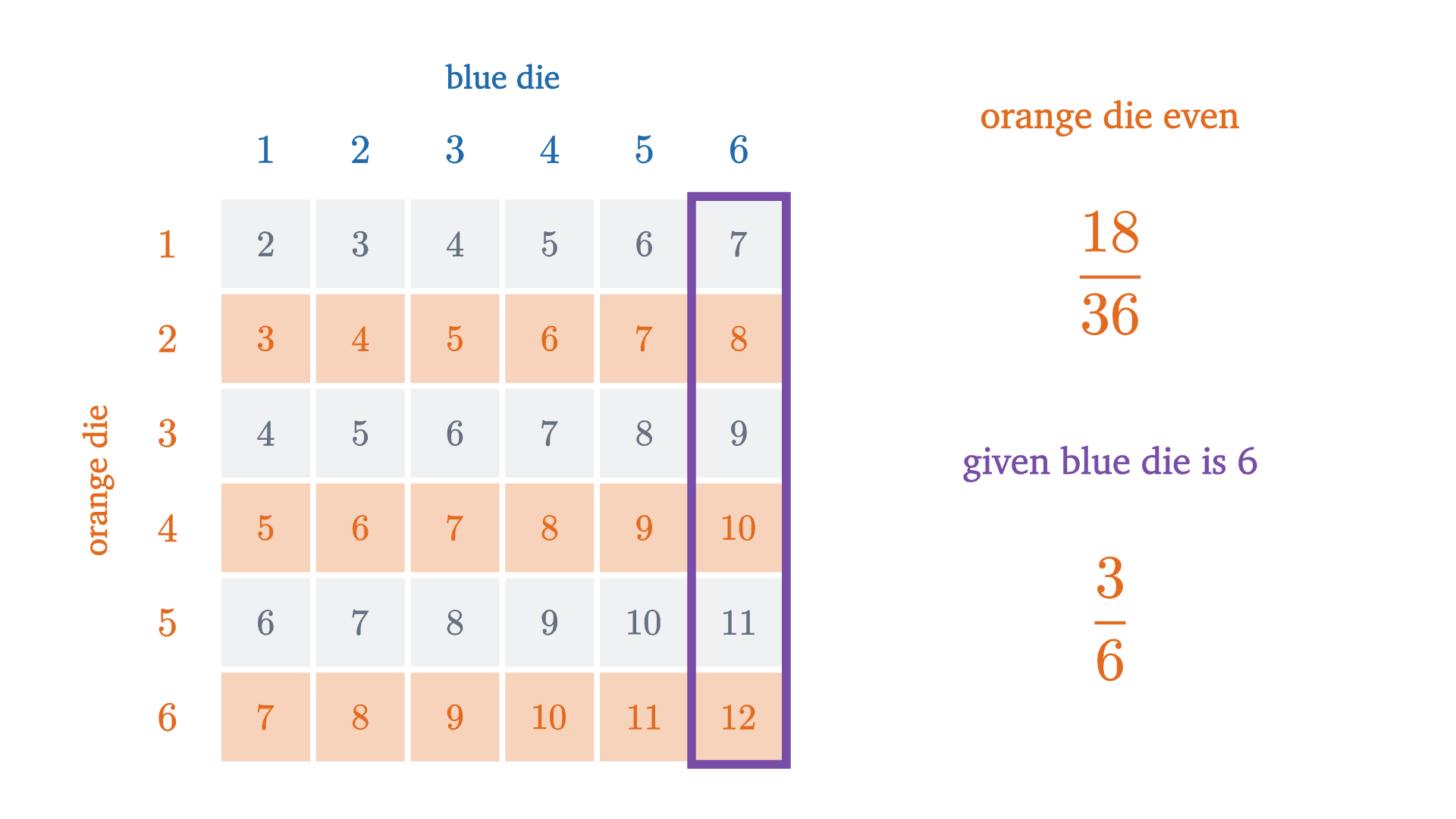
Independence on the grid. "Orange die is even" fills half of the whole grid (18 of 36 cells) and also half of the outlined column where the blue die shows 6 (3 of 6 cells), so learning that the blue die shows 6 does not change its probability.
Independence on the grid. “Orange die is even” fills half of the whole grid (18 of 36 cells) and also half of the outlined column where the blue die shows 6 (3 of 6 cells), so learning that the blue die shows 6 does not change its probability.
Monocurl source
let even_b = |a, b| mod(b, 2) == 0
let n_all = count_cells(even_b)
let n_col = count_cells(|a, b| a == 6 and mod(b, 2) == 0)
mesh base = [Headers, Lit(|a, b| 1, SLATE, 0.1)]
mesh hi = Lit(even_b, EMBER)
mesh column = Outline([
    [GX + 5 * CELL, GY, 0], [GX + 6 * CELL, GY, 0], [GX + 6 * CELL, GY + 6 * CELL, 0], [GX + 5 * CELL, GY + 6 * CELL, 0]
], PLUM, 4.5)
mesh panel = [
    center{[2.1, 1.6, 0]} Cap("orange die even", 0.82, EMBER),
    center{[2.1, 0.75, 0]} Frac(n_all, 36, 1.2, EMBER),
    center{[2.1, -0.3, 0]} Cap("given blue die is 6", 0.82, PLUM),
    center{[2.1, -1.15, 0]} Frac(n_col, 6, 1.2, EMBER)
]

Uses the shared definitions for this lesson's figures.

When $P(A \mid B) = P(A)$, the multiplication rule becomes $P(A \cap B) = P(A)\,P(B)$. That product form is symmetric in $A$ and $B$ and needs no assumption that anything is positive, so it is used as the definition.

The equivalence is one line: divide both sides of the product equation by $P(B)$, or multiply $P(A \mid B) = P(A)$ through by it. In the dice example, “doubles” and “total at least 10” were not independent: $P(A \mid B) = 1/3$ while $P(A) = 1/6$. Whether two events are independent is settled by this computation. Often we go the other way, and assume independence on physical grounds (two dice do not influence each other) in order to compute $P(A \cap B)$ by multiplying. That assumption is what justified treating the 36 cells as equally likely in the first place: $\frac16 \times \frac16 = \frac{1}{36}$.

Worked examples
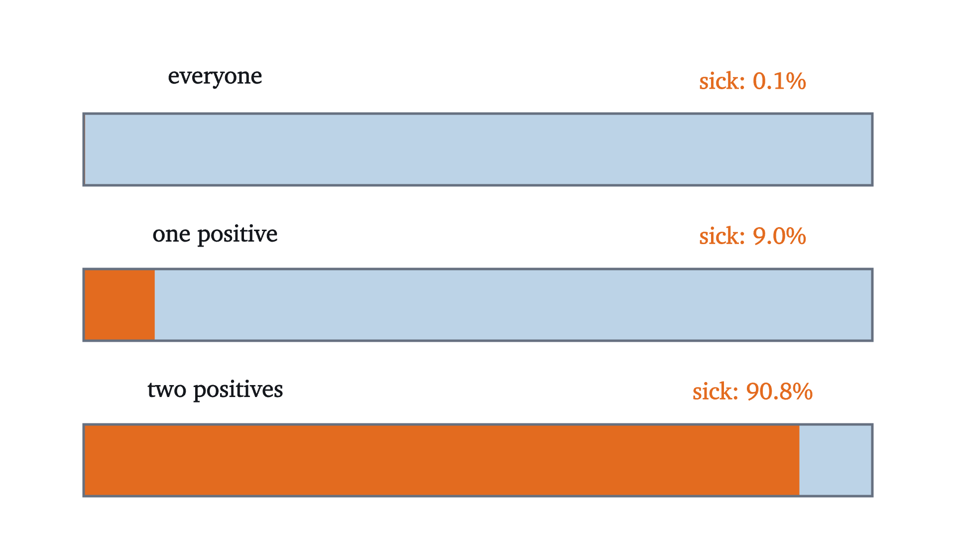
The share of sick people in three groups: everyone, those with one positive test, and those with two positive tests (assuming the two tests err independently). Each bar is a whole group, with the sick share in orange.
Monocurl source
let p0 = PREV
let p1 = post(p0)
let p2 = post(p1)
let BW = 6.6
let BL = -3.3
let Bar = |y, p, name| [
    Region([[BL, y - 0.3, 0], [BL + BW, y - 0.3, 0], [BL + BW, y + 0.3, 0], [BL, y + 0.3, 0]], tint(AZURE, 0.3)),
    Region([[BL, y - 0.3, 0], [BL + max(p * BW, 0.012), y - 0.3, 0], [BL + max(p * BW, 0.012), y + 0.3, 0], [BL, y + 0.3, 0]], EMBER),
    Outline([[BL, y - 0.3, 0], [BL + BW, y - 0.3, 0], [BL + BW, y + 0.3, 0], [BL, y + 0.3, 0]], SLATE, 2),
    center{[BL + 1.1, y + 0.58, 0]} Cap(name, 0.8),
    center{[BL + BW - 1.0, y + 0.58, 0]} Cap(str_join(["sick: ", to_string(100 * p, 1), "%%"]), 0.8, EMBER)
]
mesh bars = [
    Bar(1.0, p0, "everyone"),
    Bar(-0.3, p1, "one positive"),
    Bar(-1.6, p2, "two positives")
]

Uses the shared definitions for this lesson's figures.

Common mistakes

One more caution concerns the hypotheses of the law of total probability. If the $B_i$ overlap or fail to cover $\Omega$, the formula gives wrong answers. With two dice let $A$ be “total is 12”, $B_1$ “blue die is 6” and $B_2$ “orange die is 6”. Then $P(A \mid B_1)P(B_1) + P(A \mid B_2)P(B_2) = \frac16 \cdot \frac16 + \frac16 \cdot \frac16 = \frac{2}{36}$, while $P(A) = \frac{1}{36}$. The cell $(6,6)$ lies in both $B_1$ and $B_2$ and has been counted twice.

Stepping back

The arithmetic in the opening question is a single fraction. The difficulty is seeing that “99% accurate” describes the test’s behavior within the sick group and within the healthy group, while the question asks about the composition of the positive group, and that the two are connected only through how large the sick and healthy groups were to begin with. Bayes’ theorem is the bookkeeping for that connection.

The habit worth keeping is the one in the tree: when a conditional probability feels confusing, replace it with counts in an imagined population, split by the thing you do not know, and then collect everyone who matches what you observed. The next lesson uses the multiplication rule along a chain of events to explain another result that most people guess badly: how few people it takes before two of them share a birthday.

Check yourself

A condition affects 1% of a population. A test detects 90% of cases and gives a false positive for 10% of people without the condition. A person tests positive. Which is closest to the probability that they have the condition?

Problems

For each test problem, draw the tree for a convenient population before using the formula.

Problem 1

Two fair dice, one blue and one orange, are rolled. Find $P(\text{total} \ge 9 \mid \text{blue die shows } 5)$ and $P(\text{blue die shows } 5 \mid \text{total} \ge 9)$.

Show solutionHide solution

Let $A$ be “total at least 9” and $B$ be “blue die shows 5”. $B$ has 6 cells, $(5,1), \dots, (5,6)$, and the ones with total at least 9 are $(5,4), (5,5), (5,6)$, so $|A \cap B| = 3$ and $P(A \mid B) = 3/6 = 1/2$. For the reverse, $A$ consists of the totals 9, 10, 11, 12 with $4 + 3 + 2 + 1 = 10$ cells, so $P(B \mid A) = 3/10$. Same numerator, different denominators.

Problem 2

A condition has prevalence 2%. A test has sensitivity 95% and a false positive rate of 10%. Find the probability that a person who tests positive has the condition.

Show solutionHide solution

Per 10,000 people: 200 have the condition, of whom $0.95 \times 200 = 190$ test positive; 9,800 do not, of whom $0.10 \times 9800 = 980$ test positive. So

$$ P(\text{condition} \mid +) = \frac{190}{190 + 980} = \frac{190}{1170} \approx 0.162. $$

By the formula: $\dfrac{0.95 \times 0.02}{0.95 \times 0.02 + 0.10 \times 0.98} = \dfrac{0.019}{0.117}$, the same number.

Problem 3

Urn 1 contains 3 red balls and 1 blue ball. Urn 2 contains 1 red ball and 3 blue balls. A fair coin is flipped to choose an urn, and one ball is drawn at random from it. Find the probability that the ball is red. Given that it is red, find the probability that it came from urn 1.

Show solutionHide solution

The urns partition the possibilities, each with probability $1/2$. By the law of total probability,

$$ P(\text{red}) = \frac34 \cdot \frac12 + \frac14 \cdot \frac12 = \frac38 + \frac18 = \frac12. $$

By Bayes’ theorem, $P(\text{urn 1} \mid \text{red}) = \dfrac{3/8}{1/2} = \dfrac34$. Check with counts: run the experiment 8 times; on average urn 1 is chosen 4 times and gives 3 reds, urn 2 is chosen 4 times and gives 1 red. Of the 4 reds, 3 came from urn 1.

Problem 4

In the opening scenario (prevalence 0.001, sensitivity 0.99, false positive rate 0.01), suppose your test is negative. What is the probability that you are sick anyway?

Show solutionHide solution

Use the tree with 100,000 people. The negatives are the 1 sick person the test missed and the $99{,}900 - 999 = 98{,}901$ healthy people correctly cleared. So

$$ P(S \mid -) = \frac{1}{1 + 98{,}901} = \frac{1}{98{,}902} \approx 0.00001. $$

A negative result lowers the chance of disease from 1 in 1000 to about 1 in 100,000. For a rare disease a negative from this test is far more conclusive than a positive.

Problem 5

Two fair dice are rolled. Let $B$ be “the blue die shows 3”. (a) Is $B$ independent of the event “the total is 7”? (b) Is $B$ independent of “the total is 8”? Explain the difference.

Show solutionHide solution

$P(B) = 6/36 = 1/6$. (a) “Total 7” has 6 cells, probability $1/6$. The intersection is the single cell $(3,4)$, probability $1/36$, and $\frac16 \times \frac16 = \frac{1}{36}$. Independent. (b) “Total 8” has 5 cells, probability $5/36$. The intersection is the cell $(3,5)$, probability $1/36$, but $\frac16 \times \frac{5}{36} = \frac{5}{216} \neq \frac{1}{36}$. Not independent. The difference: whatever the blue die shows, exactly one orange face completes a total of 7, so knowing the blue face does not change the chance of a 7. For a total of 8, a blue 1 makes it impossible and any other blue face leaves one way, so the blue face does carry information.

Problem 6

A family has two children. Assume each child is equally likely to be a boy or a girl, independently. (a) Given that the older child is a girl, what is the probability that both are girls? (b) Given that at least one child is a girl, what is the probability that both are girls?

Show solutionHide solution

The sample space, listing the older child first, is $\{GG, GB, BG, BB\}$ with each outcome of probability $1/4$. (a) “Older is a girl” is $\{GG, GB\}$, and $GG$ is one of its two outcomes: $1/2$. (b) “At least one girl” is $\{GG, GB, BG\}$, and $GG$ is one of its three outcomes: $1/3$. The two conditions sound alike and are different events, of sizes 2 and 3. This is the same structure as the “at least one six” example.

Problem 7

Let $P$ be a probability measure on a finite sample space $\Omega$ and let $B$ be an event with $P(B) > 0$. Define $Q(A) = P(A \mid B)$ for every event $A$. Prove that $Q$ is a probability measure, that is, that it satisfies the three axioms: $Q(A) \ge 0$; $Q(\Omega) = 1$; and $Q(A_1 \cup A_2) = Q(A_1) + Q(A_2)$ whenever $A_1$ and $A_2$ are disjoint.

Show solutionHide solution

Nonnegativity. $Q(A) = P(A \cap B)/P(B)$ is a nonnegative number divided by a positive one. Normalization. $\Omega \cap B = B$, so $Q(\Omega) = P(B)/P(B) = 1$. Additivity. Let $A_1$ and $A_2$ be disjoint. Then $(A_1 \cup A_2) \cap B = (A_1 \cap B) \cup (A_2 \cap B)$, and the two sets on the right are disjoint because they are subsets of $A_1$ and $A_2$. By additivity of $P$,

$$ Q(A_1 \cup A_2) = \frac{P(A_1 \cap B) + P(A_2 \cap B)}{P(B)} = Q(A_1) + Q(A_2). $$

So conditioning on $B$ produces a new probability measure, and every rule proved from the axioms (the complement rule, the addition rule) holds for conditional probabilities too. For instance $P(A^c \mid B) = 1 - P(A \mid B)$.

Problem 8

For the disease with prevalence 1 in 1000, suppose a test has the same number $a$ for its sensitivity and for its probability of a correct negative on a healthy person (so its false positive rate is $1 - a$). How large must $a$ be for a positive result to mean the person is more likely sick than not?

Show solutionHide solution

By Bayes’ theorem,

$$ P(S \mid +) = \frac{0.001\,a}{0.001\,a + 0.999\,(1 - a)}. $$

This exceeds $\frac12$ exactly when the numerator exceeds the other term of the denominator: $0.001\,a > 0.999\,(1 - a)$, that is, $a > 0.999$. The test must be wrong less than once in a thousand, which is to say its error rate must be smaller than the prevalence. At $a = 0.999$ exactly, per million people there are 999 true positives and 999 false positives, and the posterior is $\frac12$. This is a useful rule of thumb: a positive result is more likely true than false only when the disease is more common than the test’s false alarms.

Shared definitions used by this lesson's figures
# house kit: prepended to every essay figure after the std imports

# palette. AZURE and EMBER are the two actors, LEAF marks an answer, ROSE a problem
let PAPER = [1, 1, 1, 1]
let INK = [0.08, 0.09, 0.11, 1]
let SLATE = [0.40, 0.44, 0.50, 1]
let MIST = [0.85, 0.86, 0.88, 1]
let AZURE = [0.13, 0.42, 0.68, 1]
let EMBER = [0.89, 0.42, 0.12, 1]
let LEAF = [0.13, 0.55, 0.36, 1]
let ROSE = [0.78, 0.22, 0.24, 1]
let PLUM = [0.47, 0.30, 0.66, 1]
let GOLD = [0.85, 0.62, 0.08, 1]

background = PAPER

# an opaque pastel of col; use for fills so overlaps do not darken
let tint = |col, amount = 0.18| [
    1 - (1 - col[0]) * amount,
    1 - (1 - col[1]) * amount,
    1 - (1 - col[2]) * amount,
    1
]

# text: Cap for labels, Note for quiet labels, Math for typeset maths
let Cap = |txt, size = 0.75, col = INK| color{col} Text(txt, size, "Charter")
let Note = |txt, size = 0.65| color{SLATE} Text(txt, size, "Charter")
let Math = |tex, size = 0.9, col = INK| color{col} Tex(tex, size)

# a paper rectangle to sit behind text that crosses lines
let Plate = |pos, size| center{pos} fill{PAPER} stroke{alpha{0} PAPER, 0} Rect(size)

# shapes with fill and stroke both set, so no stray black appears
let Pt = |pos, col = INK, r = 0.075| center{pos} fill{col} stroke{col, 1} Circle(r, 48)
let Ring = |pos, col = INK, r = 0.1, w = 3| center{pos} fill{PAPER} stroke{col, w} Circle(r, 48)
let Seg = |a, b, col = INK, w = 3| stroke{col, w} Line(a, b)
let Path = |pts, col = INK, w = 3| stroke{col, w} Polyline(pts)
let Region = |pts, col| fill{col} stroke{alpha{0} col, 0} Polygon(pts)
let Outline = |pts, col = INK, w = 3| fill{alpha{0} PAPER} stroke{col, w} Polygon(pts)
let Shape = |pts, col, amount = 0.18, w = 3| fill{tint(col, amount)} stroke{col, w} Polygon(pts)
let Disc = |pos, r, col, amount = 0.18, w = 3| center{pos} fill{tint(col, amount)} stroke{col, w} Circle(r, 96)
let Box = |pos, size, col, amount = 0.18, w = 3| center{pos} fill{tint(col, amount)} stroke{col, w} Rect(size)
# a line from a to b ending in a small solid arrowhead
let Tip = |a, b, col = INK, w = 3, head = 0.17| {
    let d = normalize([b[0] - a[0], b[1] - a[1], 0])
    let n = [-d[1], d[0], 0]
    let base = [b[0] - d[0] * head, b[1] - d[1] * head, 0]
    return [
        stroke{col, w} Line(a, base),
        fill{col} stroke{col, 1} Polygon([
            b,
            [base[0] + n[0] * head * 0.42, base[1] + n[1] * head * 0.42, 0],
            [base[0] - n[0] * head * 0.42, base[1] - n[1] * head * 0.42, 0]
        ])
    ]
}

# plots. a frame is [x0, x1, y0, y1, centre, width, height]: a data window and the scene box it fills
let Frame = |x0, x1, y0, y1, c = [0, 0, 0], w = 6.4, h = 3.6| [x0, x1, y0, y1, c, w, h]
let fx = |fr, x| fr[4][0] + (x - (fr[0] + fr[1]) / 2) * fr[5] / (fr[1] - fr[0])
let fy = |fr, y| fr[4][1] + (y - (fr[2] + fr[3]) / 2) * fr[6] / (fr[3] - fr[2])
let at = |fr, x, y| [fx(fr, x), fy(fr, y), 0]

# axes through the data origin (or the nearest edge of the window), with optional names
let Axes = |fr, x_name = "", y_name = "", col = SLATE| {
    let ox = clamp(fr[0], 0, fr[1])
    let oy = clamp(fr[2], 0, fr[3])
    var parts = [
        Tip(at(fr, fr[0], oy), [fx(fr, fr[1]) + 0.25, fy(fr, oy), 0], col, 2.5, 0.15),
        Tip(at(fr, ox, fr[2]), [fx(fr, ox), fy(fr, fr[3]) + 0.25, 0], col, 2.5, 0.15)
    ]
    if (x_name != "") {
        parts .= center{[fx(fr, fr[1]) + 0.5, fy(fr, oy), 0]} Math(x_name, 0.8, col)
    }
    if (y_name != "") {
        parts .= center{[fx(fr, ox), fy(fr, fr[3]) + 0.5, 0]} Math(y_name, 0.8, col)
    }
    return parts
}

# tick marks with numbers at the listed data values
let XTicks = |fr, xs, col = SLATE, places = 0| block {
    let oy = fy(fr, clamp(fr[2], 0, fr[3]))
    for (x in xs) {
        . Seg([fx(fr, x), oy - 0.07, 0], [fx(fr, x), oy + 0.07, 0], col, 2)
        . center{[fx(fr, x), oy - 0.33, 0]} Math(to_string(x, places), 0.72, col)
    }
}
let YTicks = |fr, ys, col = SLATE, places = 0| block {
    let ox = fx(fr, clamp(fr[0], 0, fr[1]))
    for (y in ys) {
        . Seg([ox - 0.07, fy(fr, y), 0], [ox + 0.07, fy(fr, y), 0], col, 2)
        . center{[ox - 0.36, fy(fr, y), 0]} Math(to_string(y, places), 0.72, col)
    }
}

# faint grid lines at the listed data values
let GridLines = |fr, xs, ys, col = MIST| block {
    for (x in xs) {
        . Seg(at(fr, x, fr[2]), at(fr, x, fr[3]), col, 1.5)
    }
    for (y in ys) {
        . Seg(at(fr, fr[0], y), at(fr, fr[1], y), col, 1.5)
    }
}

# the graph of f over [a, b], drawn in the frame. values are clamped to the window
let Graph = |fr, f, a, b, col = AZURE, w = 4, n = 160|
    stroke{col, w} Polyline(map(sample(a, b, n), |x| at(fr, x, clamp(fr[2], f(x), fr[3]))))

# the region between the graph of f and the x axis over [a, b]
let AreaUnder = |fr, f, a, b, col = AZURE, amount = 0.2, n = 80| {
    var pts = [at(fr, a, 0)]
    for (x in sample(a, b, n)) {
        pts .= at(fr, x, clamp(fr[2], f(x), fr[3]))
    }
    pts .= at(fr, b, 0)
    return fill{tint(col, amount)} stroke{alpha{0} col, 0} Polygon(pts)
}

let rnd = |i, salt| mod(seeded_random(i, salt) + 1, 1)

# the test in the opening question
let PREV = 0.001
let SENS = 0.99
let FPR = 0.01
# chance of the condition after a positive result, starting from chance p
let post = |p, sens = SENS, fpr = FPR| p * sens / (p * sens + (1 - p) * fpr)

# a whole number written with a comma for thousands
let commas = |n, sep = ","| {
    let k = to_int(round(n))
    if (k < 1000) {
        return to_string(k)
    }
    let r = to_int(mod(k, 1000))
    var pad = ""
    if (r < 100) {
        pad = "0"
    }
    if (r < 10) {
        pad = "00"
    }
    return str_join([to_string(to_int(k // 1000)), sep, pad, to_string(r)])
}

# the 6 by 6 grid of outcomes for two dice: blue die picks the column, orange die the row
let CELL = 0.52
let GX = -2.8
let GY = -1.95
let cell_pos = |a, b| [GX + (a - 0.5) * CELL, GY + (6.5 - b) * CELL, 0]
let Tile = |a, b, col, amount = 0.3| [
    center{cell_pos(a, b)} fill{tint(col, amount)} stroke{PAPER, 3} Rect([CELL, CELL]),
    center{cell_pos(a, b)} Math(to_string(a + b), 0.72, col)
]
let Headers = block {
    for (k in range(1, 7)) {
        . center{[GX + (k - 0.5) * CELL, GY + 6 * CELL + 0.26, 0]} Math(to_string(k), 0.8, AZURE)
        . center{[GX - 0.28, GY + (6.5 - k) * CELL, 0]} Math(to_string(k), 0.8, EMBER)
    }
    . center{[GX + 3 * CELL, GY + 6 * CELL + 0.66, 0]} Cap("blue die", 0.72, AZURE)
    . center{[GX - 0.66, GY + 3 * CELL, 0]} rotate{PI / 2} Cap("orange die", 0.72, EMBER)
}
let Lit = |pick, col, amount = 0.3| block {
    for (a in range(1, 7)) {
        for (b in range(1, 7)) {
            if (pick(a, b)) {
                . Tile(a, b, col, amount)
            }
        }
    }
}
let count_cells = |pick| {
    var n = 0
    for (a in range(1, 7)) {
        for (b in range(1, 7)) {
            if (pick(a, b)) {
                n = n + 1
            }
        }
    }
    return n
}
let Frac = |num, den, size = 1.3, col = INK| Math(str_join(["\frac{", to_string(num), "}{", to_string(den), "}"]), size, col)