
Monocurl Essays
Series Download

Double integrals: volume under a surface

Volume under a surface is a limit of sums of thin columns. Slicing turns it into two ordinary integrals, and polar coordinates handle round regions.

23 min·Early college·

AssumesSurfaces and contour maps: functions of two variablesWhat is an integral? Adding up to get areaThe fundamental theorem of calculus, explained and proved

The hill above a square of the map, replaced by 4, 16, 64 and 256 flat-topped columns, each as tall as the hill at the middle of its base. Their total volume settles toward $\frac{80}{3} \approx 26.67$.
Monocurl source
let v = View([-2.7, -0.5, 0], 1.62)
let Read = |n| [
    center{[2.6, 1.25, 0]} Note("columns", 0.76),
    center{[2.6, 0.72, 0]} Math(to_string(n * n), 1.1),
    center{[2.6, -0.2, 0]} Note("their total volume", 0.76),
    center{[2.6, -0.75, 0]} Math(to_string(midsum(n), 2), 1.2, EMBER)
]
mesh cols = Columns(v, 2)
mesh read = Read(2)

slide "refine"
    play Wait(1.2)
    for (n in [4, 8, 16]) {
        read = []
        play Fade(0.3, [&read])
        cols = Columns(v, n)
        read = Read(n)
        play Fade(0.7)
        play Wait(1)
    }
    play Wait(1.2)

Uses the shared definitions for this lesson's figures.

How much rock is in a hill? For a box the answer is length times width times height, but a hill has a different height over every point of its base, so there is no single height to multiply by.

The area under a curve has no single height either, and the integral handles it by cutting the base into slices, treating the height as constant on each slice, adding the rectangles, and taking a limit. We will do the same with one more dimension, and find that the volume under a surface can be computed with two ordinary one-variable integrals, one inside the other.

Our hill is the one from the lesson on contour maps. At the map position $x$ kilometers east and $y$ kilometers north of a marker post, its height in hundreds of meters is

$$ f(x, y) = 6 + 3x - x^3 - y^2. $$

We want the volume of rock between the map plane $z = 0$ and the hill, above the square $0 \le x \le 2$, $-1 \le y \le 1$. The summit, at $(1, 0)$ with height 8, is over the center of this square. Our unit of volume is a box 1 km by 1 km and one height unit (100 m) tall, which is a tenth of a cubic kilometer.

Four columns by hand

Start as coarsely as possible. Cut the square base into four cells, each 1 km on a side, and over each cell pretend the hill is flat, at the height it has above the middle of the cell.

  1. The piece of the hill above the square. The base is at height 0 and the summit at height 8.
  2. Cut the base into four cells, 1 km on a side, and read the height of the hill above the middle of each cell.
  3. Replace the hill over each cell by a flat-topped column of that height. A column’s volume is its height times its base area, 1.
  4. Add the four volumes: 7.125 + 6.875 + 7.125 + 6.875 = 28.
The first estimate: four square cells, the height of the hill above the middle of each, and four columns of those heights with total volume 28.
Monocurl source
let v = View([-2.83, -0.5, 0], 1.35)
let fm = Frame(0, 2, -1, 1, [2.3, 0.3, 0], 2.3, 2.3)
mesh solid = [Walls(v), Terrain(v)]
mesh scales = Scales(v)
mesh mapm = block {
    . stroke{alpha{0} PAPER, 0} point_map{|p| at(fm, p[0], p[1])} ColorGrid(|p, idx| land(p[0], p[1], 0.5), [X0, X1, 41], [Y0, Y1, 41], 1)
    . Outline([at(fm, 0, -1), at(fm, 2, -1), at(fm, 2, 1), at(fm, 0, 1)], SLATE, 2.5)
    for (x in [0, 1, 2]) {
        . center{[fx(fm, x), fy(fm, -1) - 0.28, 0]} Math(to_string(x), 0.7, SLATE)
    }
    for (y in [-1, 0, 1]) {
        . center{[fx(fm, 0) - 0.3, fy(fm, y), 0]} Math(to_string(y), 0.7, SLATE)
    }
    . center{[2.3, 1.75, 0]} Note("the same square on the map", 0.72)
}
mesh cells = []
mesh total = []

slide "The piece of the hill above the square. The base is at height 0 and the summit at height 8."
    play Fade(0.6)

slide "Cut the base into four cells, 1 km on a side, and read the height of the hill above the middle of each cell."
    cells = block {
        . Seg(at(fm, 1, -1), at(fm, 1, 1), SLATE, 2.5)
        . Seg(at(fm, 0, 0), at(fm, 2, 0), SLATE, 2.5)
        for (x in [0.5, 1.5]) {
            for (y in [-0.5, 0.5]) {
                . Pt(at(fm, x, y), INK, 0.06)
                . center{[fx(fm, x), fy(fm, y) + 0.27, 0]} Math(to_string(hill(x, y), 3), 0.72, INK)
            }
        }
    }
    play Fade(0.7, [&cells])

slide "Replace the hill over each cell by a flat-topped column of that height. A column's volume is its height times its base area, 1."
    solid = Columns(v, 2)
    play Fade(0.8, [&solid])

slide "Add the four volumes: 7.125 + 6.875 + 7.125 + 6.875 = 28."
    total = center{[2.3, -1.55, 0]} Math(str_join(["\text{total volume } ", to_string(midsum(2), 0)]), 0.9, EMBER)
    play Fade(0.5, [&total])

Uses the shared definitions for this lesson's figures.

The middles of the cells are $(0.5, \pm 0.5)$ and $(1.5, \pm 0.5)$, and the heights there are

$$ f(0.5, \pm 0.5) = 6 + 1.5 - 0.125 - 0.25 = 7.125, \qquad f(1.5, \pm 0.5) = 6 + 4.5 - 3.375 - 0.25 = 6.875. $$

Each column stands on a base of area 1, so its volume is its height, and the four volumes add to 28. Measuring at the middle of each cell was a choice, and a different choice gives a different number.

Pause and try

Keep the same four cells, but give each column the height of the hill above the cell’s southwest corner instead of its middle. What total volume do you get? Which of the two estimates do you trust more, and why?

Show answerHide answer

The southwest corners are $(0, -1)$, $(1, -1)$, $(0, 0)$ and $(1, 0)$, with heights $f = 5, 7, 6, 8$. The total is $26$. A middle is a fairer representative of a cell than a corner, where the hill is not typical of the cell (one of these corners is the summit itself). But neither estimate comes with a guarantee. So far the answer is somewhere around 26 to 28.

Finer columns, and what the volume is

Two estimates that disagree by 2 are not an answer. The remedy is the one-variable remedy: make the cells smaller, so that the hill has less room to vary over each one. With $n$ cells along each side there are $n^2$ columns, each on a base of area $\frac{2}{n} \cdot \frac{2}{n}$, and using middles again the totals are

cells along each sidecolumnstotal volume
2428
41627
86426.75
1625626.6875

The animation at the top shows these four stages. The steps down shrink by a factor of 4 each time: $1$, then $0.25$, then $0.0625$. If that continues, the remaining steps add up to about $0.02$, which predicts a limit of $26\frac{2}{3}$.

We have not yet said what “the volume of the hill” means, since length times width times height applies to boxes only. As with area in one variable, the volume is defined to be the number these sums close in on, provided they close in on a single number however the cells and sample points are chosen.

Each term $f(x_{ij}^*, y_{ij}^*)\,\Delta A_{ij}$ is the volume of one column: height times base area. “Any choice of sample points” covers both the middles and the corners from the exercise, and demands that in the limit they agree. The symbol $dA$ recalls the base area $\Delta A_{ij}$.

When $f \ge 0$, the number $\iint_R f\,dA$ is what we mean by the volume under the graph of $f$ over $R$. Where $f$ is negative its columns count negatively, as area below the axis does in one variable.

The definition leaves open whether the limit exists. For the functions we care about it does.

We use this theorem without proof. Its proof is the two-variable version of the one-variable argument: on a closed rectangle a continuous function is uniformly continuous, so once the cells are small enough, $f$ varies by less than any prescribed amount over every cell at once, and that traps all the Riemann sums in a narrow band.

So the hill has a volume. The definition is little help in finding it, since nobody wants to sum $n^2$ columns and take a limit.

Slabs: the volume as an integral of areas

Take all the columns that share one value of $x$. They stand in a row running south to north, and together they approximate a thin slab of the hill: the part between two vertical planes $x = \text{const}$, close together. A slab’s volume is close to its thickness times the area of its face, and the area of its face is a one-variable problem.

Cut the hill with the vertical plane at a fixed $x$. The cut face is the region under the curve $z = f(x, y)$, where now only $y$ varies, from $-1$ to $1$. Its area is an ordinary integral:

$$ A(x) = \int_{-1}^{1} f(x, y)\,dy. $$

Pause and try

Find the area of the cut face through the summit: compute $A(1) = \int_{-1}^{1} f(1, y)\,dy$. Then find $A(x)$ for a general $x$, remembering that $x$ is a constant while you integrate in $y$.

Show answerHide answer

At $x = 1$ the height is $f(1, y) = 8 - y^2$, with antiderivative $8y - \frac{y^3}{3}$, so $A(1) = \left(8 - \frac13\right) - \left(-8 + \frac13\right) = 16 - \frac23 = \frac{46}{3} \approx 15.33$. In general, writing $g(x) = 6 + 3x - x^3$ for the part that does not involve $y$, the height is $g(x) - y^2$ and $A(x) = 2g(x) - \frac23 = \frac{34}{3} + 6x - 2x^3$.

The step from antiderivative to area is the fundamental theorem of calculus: if $F' = f$ on $[a, b]$ and $f$ is continuous, then $\int_a^b f = F(b) - F(a)$.

Now sweep the cutting plane from $x = 0$ to $x = 2$. A slab of thickness $\Delta x$ at position $x$ has volume about $A(x)\,\Delta x$, and adding slabs is again a Riemann sum, this time for the one-variable function $A$.

A vertical plane sweeps east across the hill. The orange face is the cross-section at $x$, with area $A(x)$, plotted on the right. The volume passed so far is the area under the graph of $A$ up to $x$, and it reaches $\frac{80}{3} \approx 26.67$ at $x = 2$.
Monocurl source
let v = View([-3.2, -0.5, 0], 1.4)
let fa = Frame(0, 2, 0, 16, [2.3, -0.55, 0], 2.1, 2.1)
let A = |x| 34 / 3 + 6 * x - 2 * x * x * x
let V = |x| 34 * x / 3 + 3 * x * x - x * x * x * x / 2
let Fill = |c| AreaUnder(fa, A, 0, c, EMBER, 0.35)
let Slab = |c| [
    SouthWall(v, c),
    Terrain(v, c),
    CutFace(v, c, tint(EMBER, 0.45), EMBER, 2.5),
    Seg(at(fa, c, 0), at(fa, c, A(c)), EMBER, 3),
    Pt(at(fa, c, A(c)), EMBER, 0.085),
    center{[1.55, 1.3, 0]} scale{1.15} color{EMBER} Number(A(c), 2),
    center{[2.95, 1.3, 0]} scale{1.15} color{INK} Number(V(c), 2)
]
mesh ghost = Outline([pr(v, [X0, Y0, 0]), pr(v, [X1, Y0, 0]), pr(v, [X1, Y1, 0]), pr(v, [X0, Y1, 0])], MIST, 2)
mesh fillm = Fill(c: 0.04)
mesh plot = [
    GridLines(fa, [0.5, 1, 1.5, 2], [5, 10, 15]),
    Axes(fa, "", ""),
    XTicks(fa, [1, 2]),
    center{[fx(fa, 1.5), fy(fa, 0) - 0.33, 0]} Math("x", 0.8, SLATE),
    YTicks(fa, [5, 10, 15]),
    Graph(fa, A, 0, 2, EMBER, 3.5),
    center{[1.55, 1.75, 0]} Note("face area A(x)", 0.72),
    center{[2.95, 1.75, 0]} Note("volume so far", 0.72)
]
mesh slab = Slab(c: 0.04)

slide "sweep"
    play Wait(0.8)
    fillm.c = 2
    slab.c = 2
    play Lerp(6.5, [&fillm, &slab], linear)
    play Wait(1.8)

Uses the shared definitions for this lesson's figures.

So the volume should be the integral of the face areas:

$$ \int_0^2 A(x)\,dx = \int_0^2 \left(\frac{34}{3} + 6x - 2x^3\right) dx = \left[\frac{34}{3}x + 3x^2 - \frac{x^4}{2}\right]_0^2 = \frac{68}{3} + 12 - 8 = \frac{80}{3}. $$

That is $26\frac{2}{3}$, the value the column sums were heading for: about $2.67$ cubic kilometers of rock.

Written without the intermediate name $A$, the computation is an iterated integral,

$$ \int_0^2 \left( \int_{-1}^{1} f(x, y)\,dy \right) dx, $$

read from the inside out: integrate in $y$ with $x$ held constant, then integrate the result in $x$.

The other order, and Fubini’s theorem

We could just as well cut with planes of constant $y$ and sweep from south to north.

Pause and try

Do it. Compute the face area $B(y) = \int_0^2 f(x, y)\,dx$, with $y$ held constant, and then $\int_{-1}^{1} B(y)\,dy$. Before you start: must the answer be $\frac{80}{3}$ again?

Show answerHide answer

With $y$ constant, an antiderivative of $6 + 3x - x^3 - y^2$ in $x$ is $6x + \frac32 x^2 - \frac14 x^4 - y^2 x$, so $B(y) = 12 + 6 - 4 - 2y^2 = 14 - 2y^2$. Then $\int_{-1}^{1} (14 - 2y^2)\,dy = 28 - \frac43 = \frac{80}{3}$. It had better be the same, since both computations measure the same rock.

The two answers agree, and the reason is visible at the level of columns. A Riemann sum is a sum of numbers laid out in a grid, one for each cell. You may add a grid of numbers row by row or column by column, and the grand total is the same.

  1. Sixteen columns, each on a base half a kilometer on a side. Their volumes total 27.
  2. Group them by x. Each group of four is a slab across the hill, and the four slab volumes add to 27.
  3. Put them back and group by y instead. These four slabs run along the hill, and their volumes also add to 27.
The sixteen columns of the second estimate, grouped two ways. Pulled apart by $x$ they form four slabs across the hill; pulled apart by $y$ they form four slabs along it. Either way the slab volumes add to 27.
Monocurl source
let S = 1.5
let AZ = 0.2
let EL = 0.65
# the block stays centered while its slabs are pulled apart
let Cols = |gx, gy| Columns(View([-2.37 - 1.5 * S * (gx * cos(AZ) + gy * sin(AZ)), -0.49 - 1.5 * S * sin(EL) * (gy * cos(AZ) - gx * sin(AZ)), 0], S, AZ, EL), 4, gx, gy)
let slab_x = |i| 0.25 * sum(map([-0.75, -0.25, 0.25, 0.75], |y| hill(0.25 + 0.5 * i, y)))
let slab_y = |j| 0.25 * sum(map([0.25, 0.75, 1.25, 1.75], |x| hill(x, -0.75 + 0.5 * j)))
let List = |title, f, col| block {
    . center{[2.85, 1.6, 0]} Note(title, 0.74)
    for (k in range(0, 4)) {
        . center{[2.85, 1.1 - 0.47 * k, 0]} Math(to_string(f(k), 2), 0.85, col)
    }
    . Seg([2.3, -0.6, 0], [3.4, -0.6, 0], SLATE, 2)
    . center{[2.85, -0.95, 0]} Math(to_string(f(0) + f(1) + f(2) + f(3), 2), 0.95, INK)
}
mesh cols = Cols(gx: 0, gy: 0)
mesh list = [
    center{[2.85, 0.75, 0]} Note("columns", 0.74),
    center{[2.85, 0.25, 0]} Math("16", 0.95, INK),
    center{[2.85, -0.45, 0]} Note("total volume", 0.74),
    center{[2.85, -0.95, 0]} Math(to_string(midsum(4), 2), 0.95, INK)
]

slide "Sixteen columns, each on a base half a kilometer on a side. Their volumes total 27."
    play Fade(0.6)

slide "Group them by x. Each group of four is a slab across the hill, and the four slab volumes add to 27."
    list = []
    play Fade(0.3, [&list])
    cols.gx = 0.28
    play Lerp(1.4, [&cols])
    list = List("slabs by x", slab_x, EMBER)
    play Fade(0.5, [&list])

slide "Put them back and group by y instead. These four slabs run along the hill, and their volumes also add to 27."
    list = []
    play Fade(0.3, [&list])
    cols.gx = 0
    play Lerp(1, [&cols])
    cols.gy = 0.24
    play Lerp(1.4, [&cols])
    list = List("slabs by y", slab_y, AZURE)
    play Fade(0.5, [&list])

Uses the shared definitions for this lesson's figures.

For finite sums that settles it. For integrals a limit is involved, and the statement becomes a theorem, named for Guido Fubini.

We cite this theorem; here is the reason it is true and what a full proof adds. Take a Riemann sum with sample points on a grid, $(x_i^*, y_j^*)$, and group it by $x$:

$$ \sum_{i} \sum_{j} f(x_i^*, y_j^*)\,\Delta y_j\,\Delta x_i = \sum_i \left( \sum_j f(x_i^*, y_j^*)\,\Delta y_j \right) \Delta x_i. $$

The inner sum is a one-variable Riemann sum for $A(x_i^*) = \int_c^d f(x_i^*, y)\,dy$, so it is close to $A(x_i^*)$, and then the outer sum is close to $\sum_i A(x_i^*)\,\Delta x_i$, a Riemann sum for $\int_a^b A(x)\,dx$. That is the slab picture. What is missing is control of the word “close”: the inner sums must be within $\varepsilon$ of $A(x_i^*)$ for every $i$ at once, with one mesh serving all of them, or the errors could add up. Uniform continuity of $f$ on $R$ supplies that, and also shows that $A$ is continuous, so that the outer integral exists.

Without the hypothesis the two orders can disagree. For $f(x, y) = \dfrac{x^2 - y^2}{(x^2 + y^2)^2}$ on the square $0 \le x \le 1$, $0 \le y \le 1$, integrating in $y$ first gives $\frac{\pi}{4}$ and integrating in $x$ first gives $-\frac{\pi}{4}$. This function is unbounded near the origin, so it is not continuous on the closed square. The last problem works through it.

Regions that are not rectangles

Suppose the base is a region $D$ with curved sides. The definition extends with a simple device: enclose $D$ in a rectangle $R$, and let $\tilde f$ equal $f$ on $D$ and $0$ everywhere else in $R$. Columns outside $D$ then have height 0.

The slab picture still tells us how to compute it. Take $D$ to be the region between the parabola $y = x^2$ and the line $y = x$, which cross at $(0, 0)$ and $(1, 1)$. Fix $x$ between 0 and 1. The slice of $D$ at that $x$ is the segment from the parabola up to the line, so the face of the slab has area $\int_{x^2}^{x} f(x, y)\,dy$. The limits now depend on $x$, which is harmless, because $x$ is a constant during the inner integration.

  1. Fix x. The slice of the region runs in y from the parabola, y = x², up to the line, y = x.
  2. Or fix y. The slice runs in x from the line, x = y, across to the parabola, x = √y.
The region between $y = x^2$ and $y = x$, sliced two ways: vertically at a fixed $x$, and horizontally at a fixed $y$.
Monocurl source
let fr = Frame(0, 1.1, 0, 1.1, [-1.45, -0.2, 0], 3.2, 3.2)
let reg = block {
    var pts = []
    for (x in sample(0, 1, 40)) { pts .= at(fr, x, x * x) }
    . Region(pts, tint(LEAF, 0.25))
}
mesh plot = [
    reg,
    GridLines(fr, [0.25, 0.5, 0.75, 1], [0.25, 0.5, 0.75, 1]),
    Axes(fr, "x", "y"),
    XTicks(fr, [0.5, 1], SLATE, 1),
    YTicks(fr, [0.5, 1], SLATE, 1),
    Graph(fr, |x| x * x, 0, 1.04, PLUM, 3.5),
    Seg(at(fr, 0, 0), at(fr, 1.04, 1.04), AZURE, 3.5),
    center{at(fr, 0.38, 0.62)} Math("y = x", 0.8, AZURE),
    center{at(fr, 0.63, 0.13)} Math("y = x^2", 0.8, PLUM)
]
let VStrip = |x| [
    Seg(at(fr, x, x * x), at(fr, x, x), EMBER, 6),
    Pt(at(fr, x, x * x), EMBER, 0.08),
    Pt(at(fr, x, x), EMBER, 0.08),
    Seg(at(fr, x, 0), at(fr, x, x * x), EMBER, 1.5)
]
let HStrip = |y| [
    Seg(at(fr, y, y), at(fr, sqrt(y), y), EMBER, 6),
    Pt(at(fr, y, y), EMBER, 0.08),
    Pt(at(fr, sqrt(y), y), EMBER, 0.08),
    Seg(at(fr, 0, y), at(fr, y, y), EMBER, 1.5)
]
mesh strip = []
mesh notes = []

slide "Fix x. The slice of the region runs in y from the parabola, y = x², up to the line, y = x."
    strip = VStrip(x: 0.3)
    play Fade(0.5, [&strip])
    strip.x = 0.8
    play Lerp(2, [&strip])
    notes = [
        center{[2.2, 0.9, 0]} Note("y first, then x", 0.74),
        center{[2.2, 0.1, 0]} Math("\int_0^1 \!\! \int_{x^2}^{x} f\,dy\,dx", 0.95, INK)
    ]
    play Fade(0.5, [&notes])

slide "Or fix y. The slice runs in x from the line, x = y, across to the parabola, x = √y."
    notes = []
    strip = []
    play Fade(0.4, [&notes, &strip])
    strip = HStrip(y: 0.2)
    play Fade(0.5, [&strip])
    strip.y = 0.8
    play Lerp(2, [&strip])
    notes = [
        center{[2.2, 0.9, 0]} Note("x first, then y", 0.74),
        center{[2.2, 0.1, 0]} Math("\int_0^1 \!\! \int_{y}^{\sqrt{y}} f\,dx\,dy", 0.95, INK)
    ]
    play Fade(0.5, [&notes])

Uses the shared definitions for this lesson's figures.

This is also cited. It does not follow at once from the version for rectangles, because $\tilde f$ jumps from $f$ to 0 across the boundary of $D$ and so is not continuous on $R$. The extra ingredient is that the boundary curves are thin: they can be covered by cells of total area as small as we like, so the columns that straddle the boundary contribute nothing in the limit.

Round regions and the polar area element

Some regions resist both slicings. Take the dome $z = 1 - x^2 - y^2$ over the unit disc $x^2 + y^2 \le 1$. A slice at fixed $x$ runs from $y = -\sqrt{1 - x^2}$ to $y = \sqrt{1 - x^2}$, and the square roots make the integrals unpleasant. Yet in terms of the distance $r$ from the origin, the region is just $r \le 1$ and the height is $1 - r^2$.

So describe points by polar coordinates: the distance $r \ge 0$ from the origin and the angle $\theta$ counterclockwise from the positive $x$-axis, with $x = r\cos\theta$ and $y = r\sin\theta$. In these coordinates the disc is the rectangle $0 \le r \le 1$, $0 \le \theta \le 2\pi$. It is tempting to treat $r$ and $\theta$ just as we treated $x$ and $y$.

Pause and try

The area of a region $D$ is $\iint_D 1\,dA$, since a slab of height 1 has volume equal to its base area. Test the tempting idea on the unit disc: compute $\int_0^{2\pi} \int_0^1 1\,dr\,d\theta$. What should the answer have been?

Show answerHide answer

The inner integral is 1 and the outer is $2\pi$, so the tempting formula gives $2\pi \approx 6.28$. The area of the unit disc is $\pi \approx 3.14$. The formula is wrong by a factor of 2, so $dr\,d\theta$ cannot be the area of a small piece.

To see what went wrong, look at the pieces. Cutting the $(r, \theta)$ rectangle into equal cells cuts the disc by circles and rays, and the resulting pieces of the disc are far from equal.
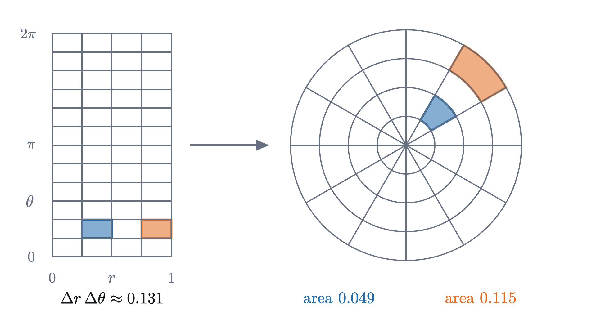
Left: the rectangle 0 \le r \le 1, 0 \le \theta \le 2\pi cut into equal cells. Right: the same cells drawn in the disc. The blue and orange cells have the same \Delta r and \Delta\theta, but in the disc the orange one, farther from the center, has more than twice the area.
Left: the rectangle $0 \le r \le 1$, $0 \le \theta \le 2\pi$ cut into equal cells. Right: the same cells drawn in the disc. The blue and orange cells have the same $\Delta r$ and $\Delta\theta$, but in the disc the orange one, farther from the center, has more than twice the area.
Monocurl source
let fq = Frame(0, 1, 0, TAU, [-2.5, 0.3, 0], 1.6, 3.0)
let C = [1.45, 0.3, 0]
let RAD = 1.55
let pol = |r, t| [C[0] + RAD * r * cos(t), C[1] + RAD * r * sin(t), 0]
let Cell = |r1, r2, t1, t2, col| {
    var pts = []
    for (t in sample(t1, t2, 12)) { pts .= pol(r2, t) }
    for (t in sample(t2, t1, 12)) { pts .= pol(r1, t) }
    return Shape(pts, col, 0.55, 2.5)
}
let cell_area = |r1, r2, dt| 0.5 * (r2 * r2 - r1 * r1) * dt
mesh rect = block {
    . Shape([at(fq, 0.25, PI / 6), at(fq, 0.5, PI / 6), at(fq, 0.5, PI / 3), at(fq, 0.25, PI / 3)], AZURE, 0.55, 2.5)
    . Shape([at(fq, 0.75, PI / 6), at(fq, 1, PI / 6), at(fq, 1, PI / 3), at(fq, 0.75, PI / 3)], EMBER, 0.55, 2.5)
    for (i in range(0, 5)) {
        . Seg(at(fq, i / 4, 0), at(fq, i / 4, TAU), SLATE, 1.5)
    }
    for (j in range(0, 13)) {
        . Seg(at(fq, 0, j * PI / 6), at(fq, 1, j * PI / 6), SLATE, 1.5)
    }
    . center{[fx(fq, 0), fy(fq, 0) - 0.28, 0]} Math("0", 0.7, SLATE)
    . center{[fx(fq, 1), fy(fq, 0) - 0.28, 0]} Math("1", 0.7, SLATE)
    . center{[fx(fq, 0.5), fy(fq, 0) - 0.3, 0]} Math("r", 0.8, SLATE)
    . center{[fx(fq, 0) - 0.28, fy(fq, 0), 0]} Math("0", 0.7, SLATE)
    . center{[fx(fq, 0) - 0.28, fy(fq, PI), 0]} Math("\pi", 0.7, SLATE)
    . center{[fx(fq, 0) - 0.32, fy(fq, TAU), 0]} Math("2\pi", 0.7, SLATE)
    . center{[fx(fq, 0) - 0.3, fy(fq, PI / 2), 0]} Math("\theta", 0.8, SLATE)
}
mesh disc = block {
    . Cell(0.25, 0.5, PI / 6, PI / 3, AZURE)
    . Cell(0.75, 1, PI / 6, PI / 3, EMBER)
    for (i in range(1, 5)) {
        . center{C} fill{alpha{0} PAPER} stroke{SLATE, 1.5} Circle(RAD * i / 4, 96)
    }
    for (j in range(0, 12)) {
        . Seg(C, pol(1, j * PI / 6), SLATE, 1.5)
    }
}
mesh arrow = Tip([-1.45, 0.3, 0], [-0.4, 0.3, 0], SLATE, 2.5, 0.16)
mesh legend = [
    center{[-2.5, -1.75, 0]} Math(str_join(["\Delta r\,\Delta\theta \approx ", to_string(0.25 * PI / 6, 3)]), 0.78, INK),
    center{[0.55, -1.75, 0]} Math(str_join(["\text{area } ", to_string(cell_area(0.25, 0.5, PI / 6), 3)]), 0.78, AZURE),
    center{[2.45, -1.75, 0]} Math(str_join(["\text{area } ", to_string(cell_area(0.75, 1, PI / 6), 3)]), 0.78, EMBER)
]

Uses the shared definitions for this lesson's figures.

The Riemann sum must weight each column by the true area of its base, so we need the area of one polar cell.
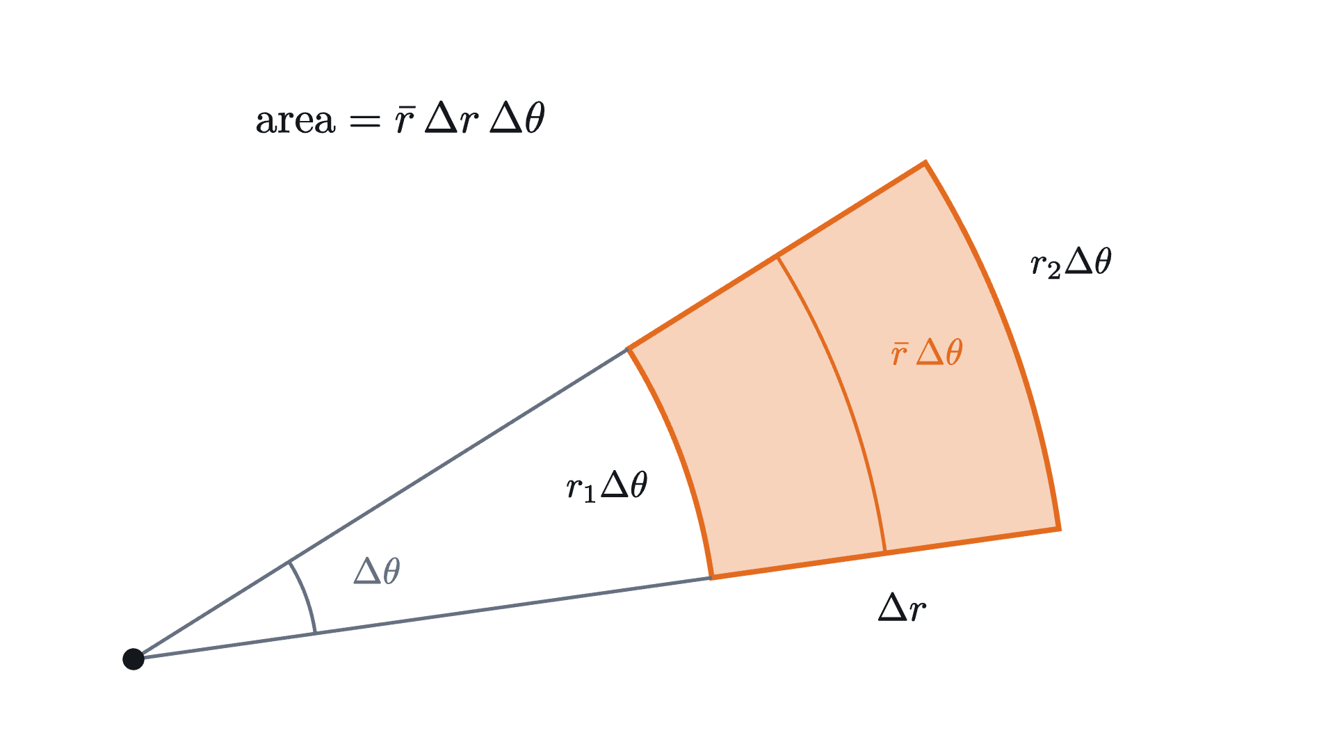
One polar cell, between the circles of radius r_1 and r_2 and two rays an angle \Delta\theta apart. Its area is \Delta r times the length \bar r\,\Delta\theta of the arc through its middle.
One polar cell, between the circles of radius $r_1$ and $r_2$ and two rays an angle $\Delta\theta$ apart. Its area is $\Delta r$ times the length $\bar r\,\Delta\theta$ of the arc through its middle.
Monocurl source
let O = [-3.2, -1.7, 0]
let T1 = 0.14
let T2 = 0.56
let R1 = 3.5
let R2 = 5.6
let RM = (R1 + R2) / 2
let P = |r, t| [O[0] + r * cos(t), O[1] + r * sin(t), 0]
let ArcPts = |r, a, b| map(sample(a, b, 30), |t| P(r, t))
mesh cell = block {
    var pts = ArcPts(R2, T1, T2)
    for (p in ArcPts(R1, T2, T1)) { pts .= p }
    . Shape(pts, EMBER, 0.3, 3)
}
mesh rays = [
    Seg(O, P(R1, T1), SLATE, 2),
    Seg(O, P(R1, T2), SLATE, 2),
    Path(ArcPts(RM, T1, T2), EMBER, 2),
    Path(ArcPts(1.1, T1, T2), SLATE, 2),
    Pt(O, INK, 0.06)
]
mesh labels = [
    center{P(1.55, (T1 + T2) / 2)} Math("\Delta\theta", 0.8, SLATE),
    center{P(RM, T1) + [0.1, -0.32, 0]} Math("\Delta r", 0.85, INK),
    center{P(R1 - 0.48, (T1 + T2) / 2)} Math("r_1\Delta\theta", 0.8, INK),
    center{P(R2 + 0.5, (T1 + T2) / 2 + 0.05)} Math("r_2\Delta\theta", 0.8, INK),
    center{P(RM + 0.55, (T1 + T2) / 2 + 0.02)} Math("\bar r\,\Delta\theta", 0.8, EMBER),
    center{[-1.6, 1.55, 0]} Math("\text{area} = \bar r\,\Delta r\,\Delta\theta", 0.95, INK)
]

Uses the shared definitions for this lesson's figures.

The cell is the difference of two circular sectors. A sector of radius $r$ and angle $\Delta\theta$ is the fraction $\frac{\Delta\theta}{2\pi}$ of a full disc, so its area is $\frac{\Delta\theta}{2\pi} \cdot \pi r^2 = \frac12 r^2 \Delta\theta$. Subtracting the inner sector from the outer one,

$$ \text{area of the cell} = \frac12 r_2^2\,\Delta\theta - \frac12 r_1^2\,\Delta\theta = \frac{r_1 + r_2}{2}\,(r_2 - r_1)\,\Delta\theta = \bar r\,\Delta r\,\Delta\theta, $$

where $\bar r = \frac{r_1 + r_2}{2}$ is the radius at the middle of the cell. This is exact. A polar cell has the area of a rectangle with sides $\Delta r$ and $\bar r\,\Delta\theta$: one side is a step outward, and the other is an arc, whose length is the angle times the radius. The factor $\bar r$ is the stretching that the tempting formula ignored.

Now form a Riemann sum over polar cells, sampling $f$ at the middle of each:

$$ \sum_{i} \sum_{j} f(\bar r_i \cos\theta_j^*, \bar r_i \sin\theta_j^*)\;\bar r_i\,\Delta r_i\,\Delta\theta_j. $$

Read this as a sum over the cells of the $(r, \theta)$ rectangle, each of area $\Delta r_i\,\Delta\theta_j$. It is then an ordinary Riemann sum for the function $f(r\cos\theta, r\sin\theta)\,r$, with the extra factor $r$ inside.

What we showed: sums over polar cells are Riemann sums of $f(r\cos\theta, r\sin\theta)\,r$ on a rectangle, so they converge to the iterated integral on the right. What we did not show: that sums over curved polar cells converge to the double integral on the left, which was defined with rectangular cells. That step is part of the change of variables theorem, which we cite.

With the factor $r$ the area of the unit disc comes out right: $\int_0^{2\pi} \int_0^1 r\,dr\,d\theta = 2\pi \cdot \frac12 = \pi$.

The Gaussian integral

The factor $r$ looks like a nuisance, but here it is the reason a computation works. The bell curve $e^{-x^2}$ has no antiderivative that can be written with the usual functions (a theorem of Liouville), so the fundamental theorem cannot evaluate the area under it. Yet the total area is known exactly.

Write $I(a) = \int_{-a}^{a} e^{-x^2}\,dx$. The idea is to compute $I(a)^2$ as a volume. Because $e^{-x^2 - y^2} = e^{-x^2} e^{-y^2}$, Fubini’s theorem over the square $S_a$: $-a \le x \le a$, $-a \le y \le a$ gives

$$ \iint_{S_a} e^{-x^2 - y^2}\,dA = \int_{-a}^{a} e^{-x^2} \left( \int_{-a}^{a} e^{-y^2}\,dy \right) dx = I(a) \cdot I(a). $$

The function $e^{-x^2-y^2} = e^{-r^2}$ depends only on $r$, so discs suit it better than squares. Over the disc $D_\rho$ of radius $\rho$ centered at the origin, the factor $r$ supplies exactly the derivative of the exponent that was missing in one variable.

Pause and try

Compute $\iint_{D_\rho} e^{-x^2 - y^2}\,dA$ in polar coordinates.

Show answerHide answer

$\int_0^{2\pi} \int_0^\rho e^{-r^2}\,r\,dr\,d\theta$. Since the derivative of $-\frac12 e^{-r^2}$ is $r e^{-r^2}$, the inner integral is $\frac12\left(1 - e^{-\rho^2}\right)$, and the outer integral multiplies by $2\pi$. The result is $\pi\left(1 - e^{-\rho^2}\right)$.

The function $e^{-x^2 - y^2}$, darker where it is larger. The square of half-side $a$ contains the disc of radius $a$ and lies inside the disc of radius $a\sqrt2$, so the integral over the square, $I(a)^2$, is trapped between the integrals over the two discs. As $a$ grows all three approach $\pi$.
Monocurl source
let fg = Frame(-3.75, 3.75, -3.75, 3.75, [-1.65, 0, 0], 3.8, 3.8)
let U = 3.8 / 7.5
let heat = stroke{alpha{0} PAPER, 0} point_map{|p| at(fg, p[0], p[1])} ColorGrid(|p, idx| lerp(PAPER, [0.42, 0.40, 0.56, 1], exp(-(p[0] * p[0] + p[1] * p[1]))), [-3.75, 3.75, 91], [-3.75, 3.75, 91], 1)
let side = |a| {
    var total = 0
    for (k in range(0, 160)) {
        let x = -a + (k + 0.5) * a / 80
        total = total + exp(-x * x) * a / 80
    }
    return total
}
let Squeeze = |a| [
    center{at(fg, 0, 0)} fill{alpha{0} PAPER} stroke{EMBER, 3} Circle(a * sqrt(2) * U, 96),
    center{at(fg, 0, 0)} fill{alpha{0} PAPER} stroke{INK, 3} Rect([2 * a * U, 2 * a * U]),
    center{at(fg, 0, 0)} fill{alpha{0} PAPER} stroke{AZURE, 3} Circle(a * U, 96),
    center{[2.35, 1.0, 0]} scale{1.15} color{AZURE} Number(PI * (1 - exp(-a * a)), 4),
    center{[2.35, -0.05, 0]} scale{1.15} color{INK} Number(side(a) * side(a), 4),
    center{[2.35, -1.1, 0]} scale{1.15} color{EMBER} Number(PI * (1 - exp(-2 * a * a)), 4)
]
mesh back = [heat, Outline([at(fg, -3.75, -3.75), at(fg, 3.75, -3.75), at(fg, 3.75, 3.75), at(fg, -3.75, 3.75)], SLATE, 2)]
mesh labels = [
    center{[2.35, 1.45, 0]} Note("over the inner disc", 0.72),
    center{[2.35, 0.4, 0]} Note("over the square", 0.72),
    center{[2.35, -0.65, 0]} Note("over the outer disc", 0.72),
    center{[2.35, -1.75, 0]} Math("\pi = 3.1416\ldots", 0.8, SLATE)
]
mesh squeeze = Squeeze(a: 0.5)

slide "grow"
    play Wait(0.8)
    squeeze.a = 2.6
    play Lerp(6, [&squeeze])
    play Wait(1.8)

Uses the shared definitions for this lesson's figures.

A remark on the meaning of $\int_{-\infty}^{\infty}$. The usual definition of an improper integral lets the two ends go to infinity separately, as $\lim_{b \to \infty} \int_0^b + \lim_{a \to \infty} \int_{-a}^0$, and our theorem used a symmetric interval. Here the two agree: $e^{-x^2}$ is even, so each half is $\frac12 I(a)$ and tends to $\frac{\sqrt\pi}{2}$. Notice also that the proof never integrated over the whole plane. It compared integrals over bounded squares and discs, to which Fubini’s theorem and the polar formula apply as stated, and took one limit at the end.

This integral is the reason the normal distribution of statistics carries a $\sqrt{2\pi}$ in its formula.

Check yourself

A plate covers the disc $x^2 + y^2 \le 4$, and its density at $(x, y)$ is $\sigma(x, y)$. Which integral gives its mass $\iint_D \sigma\,dA$?

Step back. The definition of a double integral is a limit of sums of columns, and it is the definition that says what volume means and that gives the proofs something to hold on to. But every computation here went through slabs: a volume is an integral of cross-section areas, so a double integral becomes two single ones. The hard parts were choosing how to slice, which is a question about the picture of the region, and remembering that in polar coordinates a cell’s area is $r\,\Delta r\,\Delta\theta$.

Problems

The hill is $f(x, y) = 6 + 3x - x^3 - y^2$. Problems 1 and 2 are warm-ups, 3 to 5 combine ideas, and 6 and 7 go further.

Problem 1

Compute $\displaystyle\iint_R (x + 2y)\,dA$ over the rectangle $0 \le x \le 3$, $0 \le y \le 2$, in both orders.

Show solutionHide solution

$y$ first. $\int_0^2 (x + 2y)\,dy = \left[xy + y^2\right]_0^2 = 2x + 4$, and $\int_0^3 (2x + 4)\,dx = 9 + 12 = 21$. $x$ first. $\int_0^3 (x + 2y)\,dx = \left[\frac{x^2}{2} + 2xy\right]_0^3 = \frac92 + 6y$, and $\int_0^2 \left(\frac92 + 6y\right) dy = 9 + 12 = 21$. The two agree, as Fubini’s theorem requires for a continuous integrand.

Problem 2

Find the volume of the hill above the square $-1 \le x \le 1$, $-1 \le y \le 1$, which has the pass on its west edge and the summit on its east edge. Then find the average height of the hill over that square, defined as the volume divided by the area of the base.

Show solutionHide solution

Integrate in $y$ first: $\int_{-1}^{1} (6 + 3x - x^3 - y^2)\,dy = 2(6 + 3x - x^3) - \frac23$. Then in $x$ over $[-1, 1]$: the odd terms $3x$ and $x^3$ integrate to 0, leaving $\int_{-1}^{1} \left(12 - \frac23\right) dx = 24 - \frac43 = \frac{68}{3} \approx 22.67$. The base has area 4, so the average height is $\frac{17}{3} \approx 5.67$, that is, about 567 m. It lies between the lowest height on the square, 3, and the highest, 8, as an average must.

Problem 3

Let $T$ be the triangle with corners $(0, 0)$, $(1, 0)$ and $(0, 1)$. Compute $\displaystyle\iint_T (x + y)\,dA$.

Show solutionHide solution

The slanted side is the line $y = 1 - x$. For $0 \le x \le 1$ the slice at $x$ is $0 \le y \le 1 - x$. The inner integral is $\int_0^{1-x} (x + y)\,dy = x(1 - x) + \frac{(1-x)^2}{2} = \frac{1 - x^2}{2}$, after expanding: $x - x^2 + \frac12 - x + \frac{x^2}{2} = \frac12 - \frac{x^2}{2}$. Then $\int_0^1 \frac{1 - x^2}{2}\,dx = \frac12\left(1 - \frac13\right) = \frac13$.

Problem 4

Evaluate $\displaystyle\int_0^1 \left( \int_x^1 e^{y^2}\,dy \right) dx$. The inner integral cannot be done as it stands.

Show solutionHide solution

The function $e^{y^2}$ has no elementary antiderivative in $y$, so reverse the order. The limits describe the region $0 \le x \le 1$, $x \le y \le 1$: the triangle with corners $(0, 0)$, $(0, 1)$, $(1, 1)$, above the line $y = x$. Described with $y$ outermost, $y$ runs from 0 to 1 and, for each $y$, $x$ runs from 0 to $y$. The integrand is continuous, so the theorem on regions between graphs gives the same value in either order:

$$ \int_0^1 \left( \int_0^y e^{y^2}\,dx \right) dy = \int_0^1 y\,e^{y^2}\,dy = \left[\frac{e^{y^2}}{2}\right]_0^1 = \frac{e - 1}{2} \approx 0.86. $$

The inner integration in $x$ produced the factor $y$ that makes the outer integral possible.

Problem 5

Use polar coordinates to find the volume of a ball of radius $a$. (The upper half of the sphere $x^2 + y^2 + z^2 = a^2$ is the graph of $z = \sqrt{a^2 - x^2 - y^2}$ over the disc of radius $a$.)

Show solutionHide solution

The ball is two equal halves, so its volume is $2\iint_D \sqrt{a^2 - x^2 - y^2}\,dA$ over the disc $D$ of radius $a$. In polar coordinates this is

$$ 2\int_0^{2\pi} \int_0^a \sqrt{a^2 - r^2}\;r\,dr\,d\theta. $$

The derivative of $-\frac13 (a^2 - r^2)^{3/2}$ with respect to $r$ is $r\sqrt{a^2 - r^2}$, so the inner integral is $\left[-\frac13 (a^2 - r^2)^{3/2}\right]_0^a = \frac{a^3}{3}$. The outer integral multiplies by $2\pi$, and the factor 2 in front gives $\frac{4}{3}\pi a^3$. This agrees with the value Archimedes found by comparing slices.

Problem 6

The standard normal curve of statistics is $\varphi(x) = \dfrac{1}{\sqrt{2\pi}}\,e^{-x^2/2}$. Using the Gaussian integral, show that the total area under it is 1.

Show solutionHide solution

Substitute $x = \sqrt2\,u$, so $dx = \sqrt2\,du$ and $e^{-x^2/2} = e^{-u^2}$. As $x$ runs from $-a$ to $a$, $u$ runs from $-a/\sqrt2$ to $a/\sqrt2$, so

$$ \int_{-a}^{a} e^{-x^2/2}\,dx = \sqrt2 \int_{-a/\sqrt2}^{a/\sqrt2} e^{-u^2}\,du. $$

As $a \to \infty$ the right side tends to $\sqrt2 \cdot \sqrt\pi = \sqrt{2\pi}$ by the theorem. Dividing by $\sqrt{2\pi}$ gives total area 1.

Problem 7

Let $f(x, y) = \dfrac{x^2 - y^2}{(x^2 + y^2)^2}$ for $(x, y) \ne (0, 0)$. (a) Verify that $\dfrac{\partial}{\partial y}\!\left(\dfrac{y}{x^2 + y^2}\right) = f(x, y)$. (b) Use (a) to compute $\int_0^1 \left( \int_0^1 f\,dy \right) dx$. (c) Without further integration, find $\int_0^1 \left( \int_0^1 f\,dx \right) dy$. (d) Why does this not contradict Fubini’s theorem?

Show solutionHide solution

(a) By the quotient rule, $\dfrac{\partial}{\partial y}\,\dfrac{y}{x^2 + y^2} = \dfrac{(x^2 + y^2) - y \cdot 2y}{(x^2 + y^2)^2} = \dfrac{x^2 - y^2}{(x^2 + y^2)^2}$.

(b) For a fixed $x > 0$, part (a) and the fundamental theorem give $\int_0^1 f(x, y)\,dy = \left[\dfrac{y}{x^2 + y^2}\right]_{y=0}^{y=1} = \dfrac{1}{x^2 + 1}$. Then $\int_0^1 \dfrac{dx}{1 + x^2} = \arctan 1 - \arctan 0 = \dfrac{\pi}{4}$.

(c) Exchanging the names of $x$ and $y$ turns $f$ into $-f$, since the numerator changes sign and the denominator does not. So the integral in the other order is the integral in (b) with the sign reversed: $-\dfrac{\pi}{4}$.

(d) Fubini’s theorem as stated needs $f$ to be continuous on the closed square. This $f$ is not defined at the origin and is unbounded near it: along the $x$-axis $f(x, 0) = \dfrac{1}{x^2}$, which grows without limit as $x \to 0$. No value assigned at the origin can make it continuous. The hypothesis fails, so the theorem says nothing, and the two iterated integrals are free to differ.

Shared definitions used by this lesson's figures
# house kit: prepended to every essay figure after the std imports

# palette. AZURE and EMBER are the two actors, LEAF marks an answer, ROSE a problem
let PAPER = [1, 1, 1, 1]
let INK = [0.08, 0.09, 0.11, 1]
let SLATE = [0.40, 0.44, 0.50, 1]
let MIST = [0.85, 0.86, 0.88, 1]
let AZURE = [0.13, 0.42, 0.68, 1]
let EMBER = [0.89, 0.42, 0.12, 1]
let LEAF = [0.13, 0.55, 0.36, 1]
let ROSE = [0.78, 0.22, 0.24, 1]
let PLUM = [0.47, 0.30, 0.66, 1]
let GOLD = [0.85, 0.62, 0.08, 1]

background = PAPER

# an opaque pastel of col; use for fills so overlaps do not darken
let tint = |col, amount = 0.18| [
    1 - (1 - col[0]) * amount,
    1 - (1 - col[1]) * amount,
    1 - (1 - col[2]) * amount,
    1
]

# text: Cap for labels, Note for quiet labels, Math for typeset maths
let Cap = |txt, size = 0.75, col = INK| color{col} Text(txt, size, "Charter")
let Note = |txt, size = 0.65| color{SLATE} Text(txt, size, "Charter")
let Math = |tex, size = 0.9, col = INK| color{col} Tex(tex, size)

# a paper rectangle to sit behind text that crosses lines
let Plate = |pos, size| center{pos} fill{PAPER} stroke{alpha{0} PAPER, 0} Rect(size)

# shapes with fill and stroke both set, so no stray black appears
let Pt = |pos, col = INK, r = 0.075| center{pos} fill{col} stroke{col, 1} Circle(r, 48)
let Ring = |pos, col = INK, r = 0.1, w = 3| center{pos} fill{PAPER} stroke{col, w} Circle(r, 48)
let Seg = |a, b, col = INK, w = 3| stroke{col, w} Line(a, b)
let Path = |pts, col = INK, w = 3| stroke{col, w} Polyline(pts)
let Region = |pts, col| fill{col} stroke{alpha{0} col, 0} Polygon(pts)
let Outline = |pts, col = INK, w = 3| fill{alpha{0} PAPER} stroke{col, w} Polygon(pts)
let Shape = |pts, col, amount = 0.18, w = 3| fill{tint(col, amount)} stroke{col, w} Polygon(pts)
let Disc = |pos, r, col, amount = 0.18, w = 3| center{pos} fill{tint(col, amount)} stroke{col, w} Circle(r, 96)
let Box = |pos, size, col, amount = 0.18, w = 3| center{pos} fill{tint(col, amount)} stroke{col, w} Rect(size)
# a line from a to b ending in a small solid arrowhead
let Tip = |a, b, col = INK, w = 3, head = 0.17| {
    let d = normalize([b[0] - a[0], b[1] - a[1], 0])
    let n = [-d[1], d[0], 0]
    let base = [b[0] - d[0] * head, b[1] - d[1] * head, 0]
    return [
        stroke{col, w} Line(a, base),
        fill{col} stroke{col, 1} Polygon([
            b,
            [base[0] + n[0] * head * 0.42, base[1] + n[1] * head * 0.42, 0],
            [base[0] - n[0] * head * 0.42, base[1] - n[1] * head * 0.42, 0]
        ])
    ]
}

# plots. a frame is [x0, x1, y0, y1, centre, width, height]: a data window and the scene box it fills
let Frame = |x0, x1, y0, y1, c = [0, 0, 0], w = 6.4, h = 3.6| [x0, x1, y0, y1, c, w, h]
let fx = |fr, x| fr[4][0] + (x - (fr[0] + fr[1]) / 2) * fr[5] / (fr[1] - fr[0])
let fy = |fr, y| fr[4][1] + (y - (fr[2] + fr[3]) / 2) * fr[6] / (fr[3] - fr[2])
let at = |fr, x, y| [fx(fr, x), fy(fr, y), 0]

# axes through the data origin (or the nearest edge of the window), with optional names
let Axes = |fr, x_name = "", y_name = "", col = SLATE| {
    let ox = clamp(fr[0], 0, fr[1])
    let oy = clamp(fr[2], 0, fr[3])
    var parts = [
        Tip(at(fr, fr[0], oy), [fx(fr, fr[1]) + 0.25, fy(fr, oy), 0], col, 2.5, 0.15),
        Tip(at(fr, ox, fr[2]), [fx(fr, ox), fy(fr, fr[3]) + 0.25, 0], col, 2.5, 0.15)
    ]
    if (x_name != "") {
        parts .= center{[fx(fr, fr[1]) + 0.5, fy(fr, oy), 0]} Math(x_name, 0.8, col)
    }
    if (y_name != "") {
        parts .= center{[fx(fr, ox), fy(fr, fr[3]) + 0.5, 0]} Math(y_name, 0.8, col)
    }
    return parts
}

# tick marks with numbers at the listed data values
let XTicks = |fr, xs, col = SLATE, places = 0| block {
    let oy = fy(fr, clamp(fr[2], 0, fr[3]))
    for (x in xs) {
        . Seg([fx(fr, x), oy - 0.07, 0], [fx(fr, x), oy + 0.07, 0], col, 2)
        . center{[fx(fr, x), oy - 0.33, 0]} Math(to_string(x, places), 0.72, col)
    }
}
let YTicks = |fr, ys, col = SLATE, places = 0| block {
    let ox = fx(fr, clamp(fr[0], 0, fr[1]))
    for (y in ys) {
        . Seg([ox - 0.07, fy(fr, y), 0], [ox + 0.07, fy(fr, y), 0], col, 2)
        . center{[ox - 0.36, fy(fr, y), 0]} Math(to_string(y, places), 0.72, col)
    }
}

# faint grid lines at the listed data values
let GridLines = |fr, xs, ys, col = MIST| block {
    for (x in xs) {
        . Seg(at(fr, x, fr[2]), at(fr, x, fr[3]), col, 1.5)
    }
    for (y in ys) {
        . Seg(at(fr, fr[0], y), at(fr, fr[1], y), col, 1.5)
    }
}

# the graph of f over [a, b], drawn in the frame. values are clamped to the window
let Graph = |fr, f, a, b, col = AZURE, w = 4, n = 160|
    stroke{col, w} Polyline(map(sample(a, b, n), |x| at(fr, x, clamp(fr[2], f(x), fr[3]))))

# the region between the graph of f and the x axis over [a, b]
let AreaUnder = |fr, f, a, b, col = AZURE, amount = 0.2, n = 80| {
    var pts = [at(fr, a, 0)]
    for (x in sample(a, b, n)) {
        pts .= at(fr, x, clamp(fr[2], f(x), fr[3]))
    }
    pts .= at(fr, b, 0)
    return fill{tint(col, amount)} stroke{alpha{0} col, 0} Polygon(pts)
}

# the running hill: height in hundreds of meters above the point x km east and y km north
let hill = |x, y| 6 + 3 * x - x * x * x - y * y
let hill_x = |x, y| 3 - 3 * x * x
let hill_y = |x, y| -2 * y
# the square of the map this lesson works over
let X0 = 0
let X1 = 2
let Y0 = -1
let Y1 = 1
let EDGE = [0.36, 0.38, 0.34, 1]
# land color by height, shaded as if lit from the northwest
let ramp = |h| keyframe_lerp([1 -> [0.40, 0.60, 0.43, 1], 4 -> [0.66, 0.77, 0.50, 1], 6 -> [0.88, 0.82, 0.60, 1], 8 -> [0.98, 0.96, 0.92, 1]], clamp(h, 1, 8))
let LIGHT = normalize([-0.6, 0.5, 0.62])
let relief = |x, y| clamp(dot(normalize([-0.3 * hill_x(x, y), -0.3 * hill_y(x, y), 1]), LIGHT), 0, 1)
let shade = |c, s| [clamp(c[0] * s, 0, 1), clamp(c[1] * s, 0, 1), clamp(c[2] * s, 0, 1), 1]
let land = |x, y, soft = 1| shade(ramp(hill(x, y)), 1 + soft * (0.62 + 0.62 * relief(x, y) - 1))
# a view of the block from the south: [screen origin, scale, azimuth, elevation, vertical scale]
let View = |o = [-2.75, -0.42, 0], s = 1.75, az = 0.2, el = 0.65, zs = 0.16| [o, s, az, el, zs]
let pr = |v, p| [
    v[0][0] + v[1] * (p[0] * cos(v[2]) + p[1] * sin(v[2])),
    v[0][1] + v[1] * ((p[1] * cos(v[2]) - p[0] * sin(v[2])) * sin(v[3]) + p[2] * v[4] * cos(v[3])),
    0
]
let on_hill = |v, x, y| pr(v, [x, y, hill(x, y)])
# the terrain over the square, as far east as x1
let Terrain = |v, x1 = X1| stroke{alpha{0} PAPER, 0} point_map{|p| pr(v, [p[0], p[1], hill(p[0], p[1])])}
    ColorGrid(|p, idx| land(p[0], p[1]), [X0, x1, 49], [Y0, Y1, 49], 1)
# the south face of the block as far east as x1, and the cut face at x = x1
let SouthWall = |v, x1 = X1| {
    var out = []
    for (x in sample(X0, x1, 40)) { out .= pr(v, [x, Y0, hill(x, Y0)]) }
    out .= pr(v, [x1, Y0, 0])
    out .= pr(v, [X0, Y0, 0])
    return fill{[0.82, 0.78, 0.72, 1]} stroke{SLATE, 1.5} Polygon(out)
}
let CutFace = |v, x1 = X1, col = [0.72, 0.68, 0.62, 1], edge = SLATE, w = 1.5| {
    var out = []
    for (y in sample(Y0, Y1, 40)) { out .= pr(v, [x1, y, hill(x1, y)]) }
    out .= pr(v, [x1, Y1, 0])
    out .= pr(v, [x1, Y0, 0])
    return fill{col} stroke{edge, w} Polygon(out)
}
let Walls = |v| [SouthWall(v), CutFace(v)]
# one flat-topped column: south face, east face, top
let Column = |v, xa, xb, ya, yb, h, col| [
    fill{shade(col, 0.82)} stroke{EDGE, 1} Polygon([pr(v, [xa, ya, 0]), pr(v, [xb, ya, 0]), pr(v, [xb, ya, h]), pr(v, [xa, ya, h])]),
    fill{shade(col, 0.68)} stroke{EDGE, 1} Polygon([pr(v, [xb, ya, 0]), pr(v, [xb, yb, 0]), pr(v, [xb, yb, h]), pr(v, [xb, ya, h])]),
    fill{col} stroke{EDGE, 1} Polygon([pr(v, [xa, ya, h]), pr(v, [xb, ya, h]), pr(v, [xb, yb, h]), pr(v, [xa, yb, h])])
]
# n by n columns as tall as the hill at the middle of each cell, drawn back to front.
# gx and gy pull the slabs apart
let Columns = |v, n, gx = 0, gy = 0| block {
    for (jj in range(0, n)) {
        for (i in range(0, n)) {
            let j = n - 1 - jj
            let dx = (X1 - X0) / n
            let dy = (Y1 - Y0) / n
            let h = hill(X0 + (i + 0.5) * dx, Y0 + (j + 0.5) * dy)
            let xa = X0 + i * dx + i * gx
            let ya = Y0 + j * dy + j * gy
            . Column(v, xa, xa + dx, ya, ya + dy, h, ramp(h))
        }
    }
}
# the midpoint Riemann sum with n by n cells
let midsum = |n| {
    var total = 0
    let dx = (X1 - X0) / n
    let dy = (Y1 - Y0) / n
    for (i in range(0, n)) {
        for (j in range(0, n)) {
            total = total + hill(X0 + (i + 0.5) * dx, Y0 + (j + 0.5) * dy) * dx * dy
        }
    }
    return total
}
# scales along the edges of the block
let Scales = |v| block {
    for (x in [0, 1, 2]) {
        let p = pr(v, [x, Y0, 0])
        . Seg(p, [p[0], p[1] - 0.09, 0], SLATE, 2)
        . center{[p[0], p[1] - 0.31, 0]} Math(to_string(x), 0.7, SLATE)
    }
    let px = pr(v, [0.5, Y0, 0])
    . center{[px[0], px[1] - 0.31, 0]} Math("x", 0.8, SLATE)
    for (y in [-1, 0, 1]) {
        let p = pr(v, [X1, y, 0])
        . Seg(p, [p[0] + 0.09, p[1], 0], SLATE, 2)
        . center{[p[0] + 0.36, p[1] - 0.03, 0]} Math(to_string(y), 0.7, SLATE)
    }
    let py = pr(v, [X1, 0.5, 0])
    . center{[py[0] + 0.36, py[1] - 0.03, 0]} Math("y", 0.8, SLATE)
    . Seg(pr(v, [X0, Y0, 0]), pr(v, [X0, Y0, 8.6]), SLATE, 2.5)
    for (z in [2, 4, 6, 8]) {
        let p = pr(v, [X0, Y0, z])
        . Seg(p, [p[0] - 0.09, p[1], 0], SLATE, 2)
        . center{[p[0] - 0.3, p[1], 0]} Math(to_string(z), 0.7, SLATE)
    }
}