Taylor Series Are Local Microscopes

The usual formula for a Taylor series looks like a spell:

f(x)=f(a)+f'(a)(x-a)+\frac{f''(a)}{2!}(x-a)^2+\frac{f'''(a)}{3!}(x-a)^3+\cdots.

But the idea is not mysterious. A Taylor polynomial is the best local impersonation of a function by a polynomial. It starts with the value. Then it matches the slope. Then it matches the curvature. Then the rate of change of curvature, and so on.

Each term buys one more layer of local agreement.

Loading runtime...

0.00s

live slideshowessay-2026-taylor-series-are-local-microscopes-1.mcs

param higher_terms = 0.0

background = BLACK
camera = Camera(4b)

let approx = |x, higher_terms| {
    let h = higher_terms
    let x2 = x * x
    let x3 = x2 * x
    let x4 = x3 * x
    let x5 = x4 * x
    return 1 + x + h * x2 / 2 + h * h * x3 / 6 + h * h * h * x4 / 24 + h * h * h * h * x5 / 120
}

let TaylorCurve = |higher_terms| block {
    . stroke{BLUE, 3} ExplicitFunc(|x| approx(x, higher_terms), [-2.0, 1.2, 220])
}

let Diagram = |higher_terms| block {
    . stroke{GRAY, 1} Line(start: [-2.6, 0, 0], end: [2.6, 0, 0])
    . stroke{GRAY, 1} Line(start: [0, -0.5, 0], end: [0, 2.8, 0])
    . stroke{ORANGE, 2} ExplicitFunc(|x| exp(x), [-2.0, 1.2, 220])
    . TaylorCurve(higher_terms)
    . fill{WHITE} center{[0, 1, 0]} Circle(0.04)
    . color{WHITE} center{[0, -0.85, 0]} Text("match more derivatives at the point", 0.84)
}

mesh diagram = Diagram($higher_terms)

slide "add curvature"
    higher_terms = 0.45
    play Lerp(1.1)

slide "add more local data"
    higher_terms = 1.0
    play Lerp(1.5)

The orange curve is $e^x$. The blue curve is its Taylor polynomial at $0$. The first few approximations are

1+x,\quad 1+x+\frac{x^2}{2},\quad 1+x+\frac{x^2}{2}+\frac{x^3}{6}.

Near $0$, each new term makes the blue curve cling to the orange curve for longer. Far away, the agreement eventually breaks down unless enough terms are included. Taylor series are local first and global only when the function permits it.

Why the factorials appear

Suppose you want a polynomial

p(x)=c_0+c_1(x-a)+c_2(x-a)^2+c_3(x-a)^3+\cdots

to match $f$ near $a$. The value at $a$ gives $c_0=f(a)$. Differentiating once gives $p'(a)=c_1$, so $c_1=f'(a)$.

Differentiating twice gives $p''(a)=2c_2$, so $c_2=f''(a)/2$. Differentiating three times gives $p'''(a)=6c_3$, so $c_3=f'''(a)/6$.

That is all the factorials mean. The $n$th derivative of $(x-a)^n$ at $a$ is $n!$.

Local agreement has a precise meaning

Two functions can agree at a point but immediately separate. Matching the first derivative makes their difference smaller than a line near the point. Matching the second derivative makes the difference smaller than a quadratic. Matching through degree $n$ means

$$ f(x)-p_n(x) $$

has a zero of high order at $x=a$.

The polynomial is not merely close. It is close in the most locally structured way possible.

The danger of trusting too much

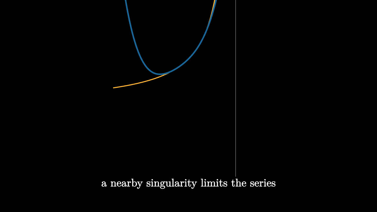
Some Taylor series behave globally. The series for $e^x$, $\sin x$, and $\cos x$ converge everywhere. Others have a limited radius of convergence. For example,

\frac{1}{1-x}=1+x+x^2+x^3+\cdots

only converges when $|x|<1$.

The reason is geometric. The function has a singularity at $x=1$. Even if you are expanding around $0$, that nearby breakdown limits how far the local microscope can see.

What a Taylor series remembers

A derivative is local data. A Taylor series is a ledger of local data. The value, slope, curvature, and every higher derivative are all stored at a single point, then used to reconstruct behavior nearby.

This is why Taylor methods are everywhere in physics and numerical computation. When a system is complicated, zoom in. If the zoom is tight enough, nonlinear behavior often becomes linear. Zoom a little less tightly, and a quadratic correction appears. Taylor series are the language of that controlled approximation.

They are not just formulas for functions we already know. They are microscopes for functions we only understand locally.